\(F=0 \rightarrow F'=1\) MOT forces

This example covers calculating the textbook example of forces in a one-dimensional MOT with an \(F=0\rightarrow F'=1\) atom. We will focus on two governing equations: the heuristic equation and the rateeq. In this example, we’ll calculate the forces using both and compare. We will also calculate the trapping frequencies and damping coefficients as well.

import numpy as np
import matplotlib.pyplot as plt
import pylcp
from pylcp.atom import atom
import scipy.constants as cts

Choose the units

Whatever units we use, let’s run numbers that are realistic for a common atom, Rb.:

rb87 = atom('87Rb')

klab = 2*np.pi*rb87.transition[1].k # Lab wavevector (without 2pi) in cm^{-1}
taulab = rb87.state[2].tau  # Lifetime of 6P_{3/2} state (in seconds)
gammalab = 1/taulab
Blab = 15 # About 15 G/cm is a typical gradient for Rb

print(klab, taulab, gammalab/2/np.pi)

80528.75481555492 2.62348e-08 6066558.277246076

As with any problem in pylcp, the units that one chooses are arbitrary. We will denote all explicit units with a subscript and all quantities where we have removed the units with an overbar, e.g. \(\bar{x} = x/x_0\). Our choice in this script will be different from the default choices of \(x_0=1/k\) and \(t_0 =1/\Gamma\). Let’s try a system where lengths are measured in terms of \(x_0 = \hbar\Gamma/\mu_B B'\) and \(t_0 = k x_0/\Gamma\). This unit system has the advantage that it measures lengths in terms of Zeeman detuning in the trap. Moreover, velocities are measured in \(\Gamma/k\). Namely,

\[v = \bar{v} \frac{x_0}{t_0} = \bar{v} \frac{\Gamma}{k}\]

From the documentation, the consistent mass scale is

\[\bar{m} = m\frac{x_0^2}{\hbar t_0}\]

# Now, here are our `natural' length and time scales:
x0 = cts.hbar*gammalab/(cts.value('Bohr magneton')*1e-4*15) # cm
t0 = klab*x0*taulab # s
mass = 87*cts.value('atomic mass constant')*(x0*1e-2)**2/cts.hbar/t0

# And now our wavevector, decay rate, and magnetic field gradient in these units:
k = klab*x0
gamma = gammalab*t0
alpha = 1.0*gamma     # The magnetic field gradient parameter

print(x0, t0, mass, k, gamma, alpha)

Alternatively, we can just use the default unit system:

# Now, here are our `natural' length and time scales:
x0 = 1/klab  # cm
t0 = taulab  # s

mass = 87*cts.value('atomic mass constant')*(x0*1e-2)**2/cts.hbar/t0

# And now our wavevector, decay rate, and magnetic field gradient in these units:
k = klab*x0
gamma = gammalab*t0
alpha = cts.value('Bohr magneton')*1e-4*15*x0*t0/cts.hbar

print(x0, t0, mass, k, gamma, alpha)

1.2417924532552691e-05 2.62348e-08 805.2161255642717 1.0 1.0 4.297436175809039e-05

It turns out there is another choice of units, useful in the next example, that works extremely well if the radiative force is the only force.

Define the problem

One has to define the Hamiltonian, laser beams, and magnetic field.

# Define the atomic Hamiltonian:
Hg, mugq = pylcp.hamiltonians.singleF(F=0, muB=1)
He, mueq = pylcp.hamiltonians.singleF(F=1, muB=1)

dijq = pylcp.hamiltonians.dqij_two_bare_hyperfine(0, 1)

ham = pylcp.hamiltonian(Hg, He, mugq, mueq, dijq, mass=mass, gamma=gamma, k=k)

det = -4.
s = 1.5

# Define the laser beams:
laserBeams = pylcp.laserBeams(
    [{'kvec':k*np.array([1., 0., 0.]), 's':s, 'pol':-1, 'delta':det*gamma},
     {'kvec':k*np.array([-1., 0., 0.]), 's':s, 'pol':-1, 'delta':det*gamma}],
    beam_type=pylcp.infinitePlaneWaveBeam
)

# Define the magnetic field:
linGrad = pylcp.magField(lambda R: -alpha*R)

Define both governing equations

We’ll add in the OBEs in a later example.

rateeq = pylcp.rateeq(laserBeams, linGrad, ham, include_mag_forces=True)
heuristiceq = pylcp.heuristiceq(laserBeams, linGrad, gamma=gamma, k=k, mass=mass)

Calculate equilibrium forces

Let’s define both positions and velocities and calculate the forces in the resulting 2D phase space

x = np.arange(-30, 30, 0.4)/(alpha/gamma)
v = np.arange(-30, 30, 0.4)

X, V = np.meshgrid(x, v)

Rvec = np.array([X, np.zeros(X.shape), np.zeros(X.shape)])
Vvec = np.array([V, np.zeros(V.shape), np.zeros(V.shape)])

rateeq.generate_force_profile(Rvec, Vvec, name='Fx', progress_bar=True)
heuristiceq.generate_force_profile(Rvec, Vvec, name='Fx', progress_bar=True)

Completed in 16.61 s.
Completed in 4.26 s.

<pylcp.common.base_force_profile at 0x7ff20bb69c90>

Now let’s plot it up, and compare to the heuristic force equation for this geometry, which is given by

\[f = \frac{\hbar k\Gamma}{2}\left(\frac{s}{1+2s +4(\Delta - k v - \mu_B B' x/\hbar)^2/\Gamma^2} - \frac{s}{1+2s +4(\Delta + k v + \mu_B B' x/\hbar)^2/\Gamma^2}\right).\]

where \(s = I/I_{\rm sat}\). Note that the quadrupole field parameter defined above \(\alpha = \mu_B B'/\hbar\)

No matter what unit system we use above, we want to measure lengths in terms of the magnetic field. Dividing by the field gradient is enough to accomplish that:

fig, ax = plt.subplots(nrows=1, ncols=2, num="Expression", figsize=(6.5, 2.75))

ax[0].plot(x*(alpha/gamma), rateeq.profile['Fx'].F[0, int(np.ceil(x.shape[0]/2)), :]/gamma/k)
ax[0].plot(x*(alpha/gamma), heuristiceq.profile['Fx'].F[0, int(np.ceil(x.shape[0]/2)), :]/gamma/k)
ax[0].plot(x*(alpha/gamma), (s/(1+2*s + 4*(det-alpha*x/gamma)**2) - s/(1+2*s + 4*(det+alpha*x/gamma)**2))/2, 'k-', linewidth=0.5)
ax[0].set_ylabel('$f/(\hbar k \Gamma)$')
ax[0].set_xlabel('$x/(\hbar \Gamma/\mu_B B\')$')
ax[0].set_xlim((-10, 10))

im1 = ax[1].contourf(X*(alpha/gamma), V, rateeq.profile['Fx'].F[0]/gamma/k, 25)
fig.subplots_adjust(left=0.08, wspace=0.2)
cb1 = plt.colorbar(im1)
cb1.set_label('$f/(\hbar k \Gamma)$')
ax[1].set_xlabel('$x/(\hbar \Gamma/\mu_B B\')$')
ax[1].set_ylabel('$v/(\Gamma/k)$')

Text(0, 0.5, '$v/(\\Gamma/k)$')

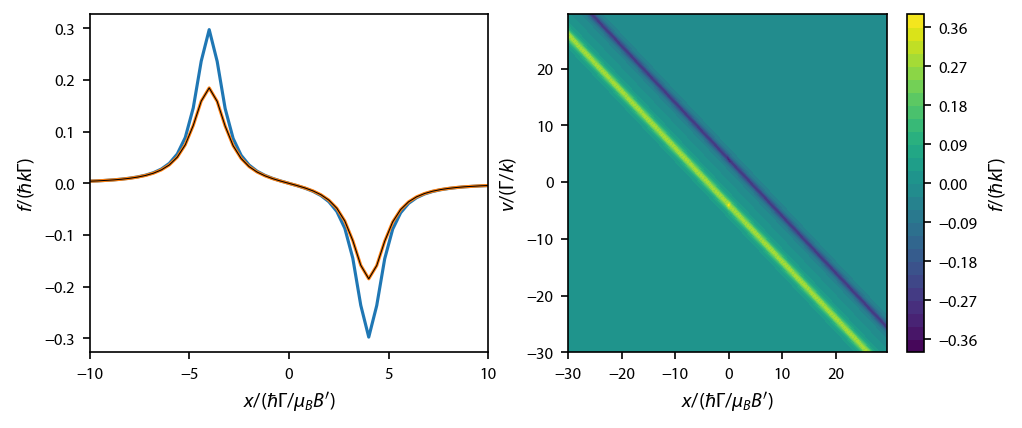
Note that heuristic equation produces less force at resonance in \(x\), because it is over-estimating the total saturation.

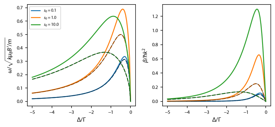
Compute the trap frequencies and damping rates

And we can compare to simple 1D theory. Let’s take the force equation above and expand it about \(x=0\) and \(v=0\). We get

\[f \approx \frac{\hbar k}{2\Gamma}\left(\frac{s \Delta}{1+2s + 4\Delta^2/\Gamma^2}\right)\left( \frac{\mu_B B'}{\hbar} x + k v\right)\]

The damping coefficient \(\beta\), most easily expressed in units of \(\hbar k^2\), and is given by

\[\frac{\beta}{\hbar k^2} = \frac{8 s \delta}{1 + 2s + 4\delta^2}\]

where \(\delta = \Delta/\Gamma\). Note that the trapping frequency is defined through

\[\ddot{x} - \frac{\beta}{m} \dot{x} + \omega^2 x = 0\]

and therefore, its square is most easily measured in units of \(k \mu_B B'/m\),

\[\frac{\omega^2}{k \mu_B B'/m} = \frac{8 s \delta}{1 + 2s + 4\delta^2}\]

Note as well that we defined \(\alpha\), the quadrupole field parameter above to be \(\alpha = \hbar \mu_B B'\).

dets = np.arange(-5, 0.05, 0.05)
intensities = np.array([0.1, 1, 10])

omega = np.zeros(intensities.shape + dets.shape)
dampingcoeff = np.zeros(intensities.shape + dets.shape)

omega_heuristic = np.zeros(intensities.shape + dets.shape)
dampingcoeff_heuristic = np.zeros(intensities.shape + dets.shape)

for ii, det in enumerate(dets):
    for jj, intensity in enumerate(intensities):
        # Define the laser beams:
        laserBeams = [None]*2
        laserBeams[0] = pylcp.laserBeam(kvec=k*np.array([1., 0., 0.]), s=intensity,
                                        pol=-1, delta=gamma*det)
        laserBeams[1] = pylcp.laserBeam(kvec=k*np.array([-1., 0., 0.]), s=intensity,
                                        pol=-1, delta=gamma*det)

        rateeq = pylcp.rateeq(laserBeams, linGrad, ham, include_mag_forces=False)
        heuristiceq = pylcp.heuristiceq(laserBeams, linGrad, gamma=gamma, mass=mass)

        omega[jj, ii] = rateeq.trapping_frequencies(axes=[0], eps=0.0002)
        dampingcoeff[jj, ii] = rateeq.damping_coeff(axes=[0], eps=0.0002)

        omega_heuristic[jj, ii] = heuristiceq.trapping_frequencies(axes=[0], eps=0.0002)
        dampingcoeff_heuristic[jj, ii] = heuristiceq.damping_coeff(axes=[0], eps=0.0002)

fig, ax = plt.subplots(1, 2, figsize=(6, 2.75))
for ii, intensity in enumerate(intensities):
    ax[0].plot(dets, omega[ii]/np.sqrt(k*alpha/mass), '-', color='C{0:d}'.format(ii),
               label='$s_0 = %.1f$'%intensity)
    ax[0].plot(dets, omega_heuristic[ii]/np.sqrt(k*alpha/mass), '--', color='C{0:d}'.format(ii))
    ax[0].plot(dets, np.sqrt(-8*dets*intensity/(1 + 2*intensity + 4*dets**2)**2), 'k-', linewidth=0.5)
    ax[1].plot(dets, dampingcoeff[ii]/k**2, '-', color='C{0:d}'.format(ii))
    ax[1].plot(dets, dampingcoeff_heuristic[ii]/k**2, '--', color='C{0:d}'.format(ii))
    ax[1].plot(dets, -8*dets*intensity/(1 + 2*intensity + 4*dets**2)**2, 'k-', linewidth=0.5)

ax[0].legend(fontsize=7, loc='upper left')
ax[1].set_ylabel('$\\beta/\hbar k^2$')
ax[0].set_ylabel('$\\omega/\sqrt{k \mu_B B\'/m}$')
ax[0].set_xlabel('$\Delta/\Gamma$')
ax[1].set_xlabel('$\Delta/\Gamma$')

fig.subplots_adjust(left=0.08, wspace=0.25)