An \(F \rightarrow F+1\) MOT with small ground state g-factor
This example covers calculating the forces in a type-I, three-dimensional MOT in a variety of different ways and comparing the various results.
[1]:
import numpy as np
import matplotlib.pyplot as plt
import pylcp
Define the problem
We’ll define the laser beams, magnetic field, and hamiltonian that we’ll use:
[2]:
# Laser beams parameters:
det = -1.5
alpha = 1.0
s = 1.0

# Define the laser beams:
laserBeams = pylcp.laserBeams(
    [{'kvec':np.array([1, 0, 0]), 's':s, 'pol':-1, 'delta':det},
     {'kvec':np.array([-1, 0, 0]), 's':s, 'pol':-1, 'delta':det}],
    beam_type=pylcp.infinitePlaneWaveBeam
)

# Actual linear gradient:
linGrad = pylcp.magField(lambda R: np.array([-alpha*R[0], np.zeros(R[1].shape),
                                             np.zeros(R[2].shape)]))

# Define the atomic Hamiltonian:
Fl = 1
Hg, muq_g = pylcp.hamiltonians.singleF(F=Fl, gF=0, muB=1)
He, muq_e = pylcp.hamiltonians.singleF(F=Fl+1, gF=1/(Fl+1), muB=1)

dijq =  pylcp.hamiltonians.dqij_two_bare_hyperfine(1, 2)

ham = pylcp.hamiltonian(Hg, He, muq_g, muq_e, dijq)
Calculate equilibrium forces
We’ll do this with two governing equations again, one rateeq and one heuristiceq for comparison.
[3]:
rateeq = pylcp.rateeq(laserBeams, linGrad, ham, svd_eps=1e-10, include_mag_forces=False)
heuristiceq = pylcp.heuristiceq(laserBeams, linGrad)
Let now define a coordinate system over which to calculate and run both:
[93]:
x = np.arange(-20+1e-9, 20.1, 0.1)
v = np.arange(-20, 20.1, 0.1)

X, V = np.meshgrid(x, v)

# Define the three-vectors used in the calculation:
Rvec = np.array([X, np.zeros(X.shape), np.zeros(X.shape)])
Vvec = np.array([V, np.zeros(V.shape), np.zeros(V.shape)])

heuristiceq.generate_force_profile(Rvec, Vvec, name='Fx')
rateeq.generate_force_profile(Rvec, Vvec, name='Fx', progress_bar=True,
                              default_axis=np.array([1., 0., 0.]))
Completed in 2:02.
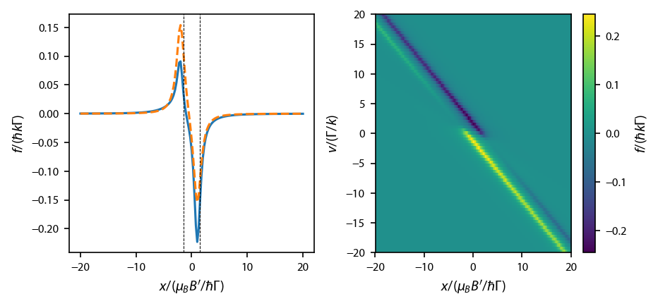
Plot up the resulting forces:
[36]:
F0 = heuristiceq.profile['Fx'].F[0]
F2 = rateeq.profile['Fx'].F[0]

# Now plot it up:
fig, ax = plt.subplots(nrows=1, ncols=2, num="Force F=2->F=3", figsize=(6.5,2.75))
im1 = ax[1].imshow(F2,extent=(np.amin(X[0,:]), np.amax(X[0,:]),
                              np.amin(V[:,0]), np.amax(V[:,0])),
                   origin='bottom',
                   aspect='auto')
cb1 = plt.colorbar(im1)
cb1.set_label('$f/(\hbar k\Gamma)$')
ax[1].set_xlabel('$x/(\mu_B B\'/\hbar \Gamma)$')
ax[1].set_ylabel('$v/(\Gamma/k)$')

ax[0].plot(x, F2[int(np.ceil(F2.shape[0]/2)),:], '-', color='C0')
ax[0].plot(x, F0[int(np.ceil(F0.shape[0]/2)),:], '--', color='C1')
ax[0].set_ylabel('$f/(\hbar k \Gamma)$')
ax[0].set_xlabel('$x/(\mu_B B\'/\hbar \Gamma)$')

ax[0].axvline(-det, color='k', linewidth=0.5, linestyle='--')
ax[0].axvline(+det, color='k', linewidth=0.5, linestyle='--')

fig.subplots_adjust(wspace=0.25)
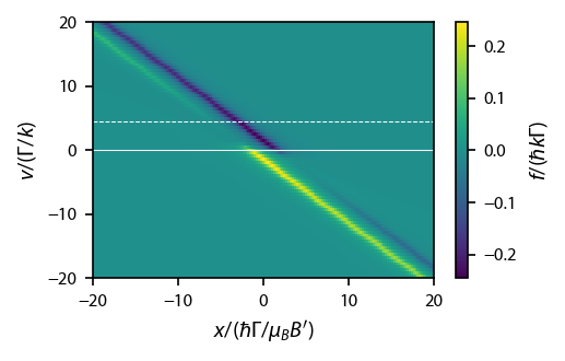
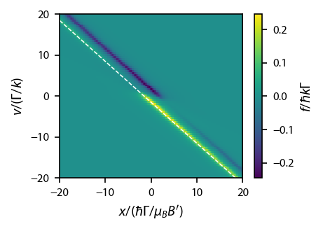
Why is the oppositely directly force dissappearing at large magnetic field?
It turns out that we are getting an interesting effect when the non-cycling transition from other beam starts to affect the population in the cycling transition ground state. Let’s start by going figuring out the line to go along for to stay in resonance with the rightward going beam.
Let’s first look at this along lines that are going along \(\hat{x}\) for various \(v\):
[168]:
v_inds = [200, 245]

fig, ax = plt.subplots(1, 1, figsize=(3.25, 2.))
im1 = ax.imshow(F2,extent=(np.amin(X[0,:]), np.amax(X[0,:]),
                           np.amin(V[:,0]), np.amax(V[:,0])),
                origin='bottom',
                aspect='auto')
cb1 = plt.colorbar(im1, ax=ax)
ax.axhline(rateeq.profile['Fx'].V[0, v_inds[0], 0], color='w', linestyle='-', linewidth=0.5)
ax.axhline(rateeq.profile['Fx'].V[0, v_inds[1], 0], color='w', linestyle='--', linewidth=0.5)
cb1.set_label('$f/(\hbar k \Gamma)$')
ax.set_xlabel('$x/(\hbar \Gamma/\mu_B B\')$')
ax.set_ylabel('$v/(\Gamma/k)$')
ax.set_ylim((np.amin(v), np.amax(v)))
fig.subplots_adjust(left=0.15, bottom=0.2, right=0.95)
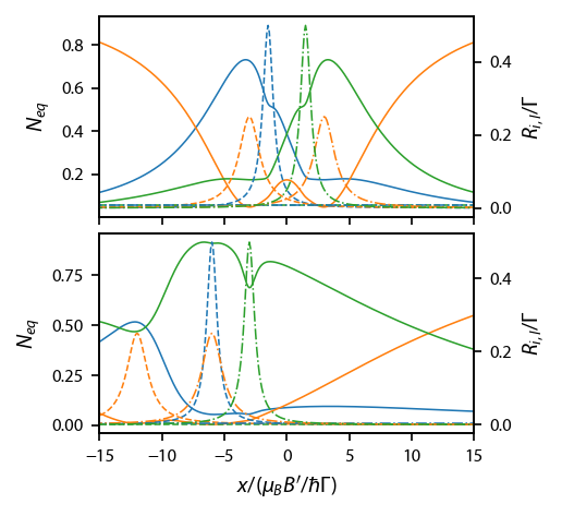
[171]:
fig, ax = plt.subplots(2, 1, figsize=(3.25, 3))
ax_twin = np.array([ax_i.twinx() for ax_i in ax])

for jj, v_ind in enumerate(v_inds):
    [ax[jj].plot(x, np.concatenate((rateeq.profile['Fx'].Neq[v_ind, x<0, ii],
                                    rateeq.profile['Fx'].Neq[v_ind, x>=0, 2-ii])),
                '-', color='C%d'%ii, linewidth=0.75) for ii in range(3)];
    [ax_twin[jj].plot(x, np.concatenate((np.sum(rateeq.profile['Fx'].Rijl['g->e'][v_ind, x<0, 0, ii, :], axis=1),
                                         np.sum(rateeq.profile['Fx'].Rijl['g->e'][v_ind, x>=0, 0, 2-ii, :], axis=1))),
                '--', color='C%d'%ii, linewidth=0.75) for ii in range(3)];
    [ax_twin[jj].plot(x, np.concatenate((np.sum(rateeq.profile['Fx'].Rijl['g->e'][v_ind, x<0, 1, ii, :], axis=1),
                                         np.sum(rateeq.profile['Fx'].Rijl['g->e'][v_ind, x>=0, 1, 2-ii, :], axis=1))),
                '-.', color='C%d'%ii, linewidth=0.75) for ii in range(3)];

    #ax[jj].axvline(-rateeq.profile['Fx'].V[0, v_ind, 0]-det, color='k', linewidth=0.5, linestyle='--')
    #ax[jj].axvline(-rateeq.profile['Fx'].V[0, v_ind, 0]+det, color='k', linewidth=0.5, linestyle='--')

    ax[jj].set_xlim(-15, 15)

[ax[ii].set_ylabel('$N_{eq}$') for ii in range(2)]
[ax_twin[ii].set_ylabel('$R_{i,l}/\Gamma$') for ii in range(2)]
ax[1].set_xlabel('$x/(\mu_B B\'/\hbar \Gamma)$')

ax[0].xaxis.set_ticklabels('');
fig.subplots_adjust(left=0.155, bottom=0.13, hspace=0.08, right=0.86)
Look along the line of resonance
Firt, compute the line where the rightward going beam is always supposed to be resonant:
[88]:
fig, ax = plt.subplots(1, 1, figsize=(3.25, 2.))
im1 = ax.imshow(F2,extent=(np.amin(X[0,:]), np.amax(X[0,:]),
                           np.amin(V[:,0]), np.amax(V[:,0])),
                origin='bottom',
                aspect='auto')
cb1 = plt.colorbar(im1, ax=ax)
ax.plot(x, det - x, 'w--', linewidth=0.75)
cb1.set_label('$f/\hbar k \Gamma$')
ax.set_xlabel('$x/(\hbar \Gamma/\mu_B B\')$')
ax.set_ylabel('$v/(\Gamma/k)$')
ax.set_ylim((np.amin(v), np.amax(v)))
fig.subplots_adjust(bottom=0.2, right=0.85)
Now, compute the parameters along that line:
[172]:
# Along the line v = delta - alpha x, we
v_path = det - alpha*x

rateeq.generate_force_profile([x, np.zeros(x.shape), np.zeros(x.shape)],
                              [v_path, np.zeros(x.shape), np.zeros(x.shape)],
                              name='res_path', default_axis=np.array([1., 0., 0.]))
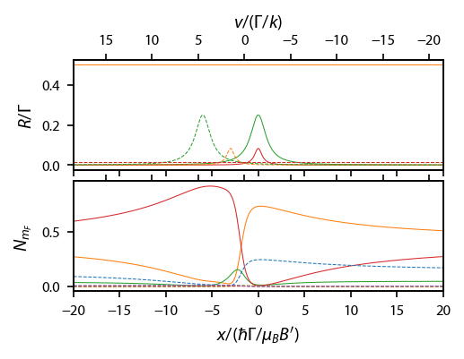
Now, plot up the scattering rate and populations along that line:
[173]:
fig, ax = plt.subplots(2, 1, figsize=(3.25, 2.5))

for ii in range(2*Fl+1):
    ax[0].plot(x, np.concatenate((rateeq.profile['res_path'].Rijl['g->e'][x<0, 0, ii, ii],
                                  rateeq.profile['res_path'].Rijl['g->e'][x>=0, 0, -1-ii, -1-ii])),
               color='C{0:d}'.format(ii+1), linewidth=0.5,
               label='$m_F= {0:d}\\rightarrow {1:d}$'.format(ii-1,ii-2))

for ii in range(2*Fl+1):
    ax[0].plot(x, np.concatenate((rateeq.profile['res_path'].Rijl['g->e'][x<0, 1, ii, ii+2],
                                  rateeq.profile['res_path'].Rijl['g->e'][x>=0, 1, -1-ii, -1-ii-2])),
               '--', color='C{0:d}'.format(ii+1), linewidth=0.5,
               label='$m_F= {0:d}\\rightarrow {1:d}$'.format(ii-1,ii))

for ii in range(2*Fl+1):
    ax[1].plot(x, np.concatenate((rateeq.profile['res_path'].Neq[x<0, ii],
                                 rateeq.profile['res_path'].Neq[x>=0, ham.ns[0]-ii-1])),
               color='C{0:d}'.format(ii+1), linewidth=0.5)

for ii in range(2*(Fl+1)+1):
    ax[1].plot(x, np.concatenate((rateeq.profile['res_path'].Neq[x<0, ham.ns[0]+ii],
                                  rateeq.profile['res_path'].Neq[x>=0, -1-ii])),
               '--', color='C{0:d}'.format(ii), linewidth=0.5)

[ax_i.set_xlim(-20, 20) for ax_i in ax];
ax_twin = [ax[ii].twiny() for ii in range(2)]
[ax_twin[ii].set_xlim(det - alpha*np.array(ax[ii].get_xlim())) for ii in range(2)];
ax_twin[1].xaxis.set_ticklabels('')
ax[0].xaxis.set_ticklabels('')
ax[1].set_xlabel('$x/(\hbar\Gamma/\mu_B B\')$')
ax_twin[0].set_xlabel('$v/(\Gamma/k)$')
ax[0].set_ylabel('$R/\Gamma$')
ax[1].set_ylabel('$N_{m_F}$')
fig.subplots_adjust(left=0.135, top=0.85)