Power broadening

Power broadening and saturation are simple effects that can replicated using the rate equations. This example shows how this works.

import numpy as np
import matplotlib.pyplot as plt
import pylcp

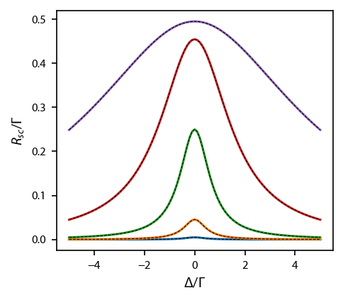
Two levels with a single laser

This is the simplest case to consider. We will plot up the scattering rate \(R_{sc} = \sum_l R_{ge,l}(N_e-N_g)\), where \(R_{ge, l}\) is the pumping rate due to laser \(l\). We can compare to the standard analytical expression for a two-level system

\[R_{sc} = \frac{1}{2}\frac{s}{1+s+4 \Delta^2/\Gamma^2},\]

which is shown in the plots as the black dashed lines.

We start by generating the Hamiltonian. Here, we use an \(F=0\rightarrow F'=1\) transition as our model system, but we will consider coupling only two of these four states together using a circularly-polarized laser beam propogating along \(\hat{z}\).

Hg, Bgq = pylcp.hamiltonians.singleF(F=0, muB=0)
He, Beq = pylcp.hamiltonians.singleF(F=1, muB=1)

dijq = pylcp.hamiltonians.dqij_two_bare_hyperfine(0, 1)

ham = pylcp.hamiltonian(Hg, He, Bgq, Beq, dijq)

Add in a constant, small magnetic field to establish a quantization axis along the \(\hat{x}\) axis:

magField = lambda R: np.array([1e-5, 0.0, 0.0])

We next run through a loop of both detuning and intensity, remaking the single laser every time. Note that it is \(\sigma^-\) polarized relative to both its \(k\) vector and the quantization axis.

# Make two independent axes: dets/betas:
dets = np.arange(-5.0, 5.1, 0.1)
intensities = np.logspace(-2, 2, 5)

fig, ax = plt.subplots(nrows=1, ncols=1)
for intensity in intensities:
    Rijl = np.zeros(dets.shape)
    Neq = np.zeros(dets.shape + (4,))
    for ii, det in enumerate(dets):
        laserBeams = pylcp.laserBeams(
            [{'kvec':np.array([1., 0, 0.]),
              's':intensity, 'pol':-1, 'delta':det}]
        )

        rateeq = pylcp.rateeq(laserBeams, magField, ham)

        Neq[ii] = rateeq.equilibrium_populations(
            np.array([0., 0., 0.]),
            np.array([0., 0., 0.]),
            0.
        )

        Rijl[ii] = np.sum(rateeq.Rijl['g->e'], axis=2)[0][0]

    ax.plot(dets, Rijl*(Neq[:, 0]-Neq[:, 1]))
    ax.plot(dets, intensity/2/(1+intensity+4*dets**2), 'k--', linewidth=0.5)

ax.set_xlabel('$\Delta/\Gamma$')
ax.set_ylabel('$R_{sc}/\Gamma$');

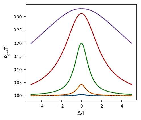
Coupling three states together

Instead of just considering a single laser coupling the \(m_F=0\) and \(m_F'=-1\), we can add in a second laser and consider coupling \(m_F=0\) to \(m_F'=+1\) as well. We add this coupling laser by adding a counter propogating laser with the same circular polarization relative to its :math:`k` vector. Relative to the quanitization axis, this laser has \(\sigma^+\) light.

We then compare to the modified analytic formula

\[R_{sc} = \frac{1}{2}\frac{s}{1+3 s/2+4 \Delta^2/\Gamma^2},\]

which is shown in the plot as black dashed lines.

# Make two independent axes: dets/betas:
fig, ax = plt.subplots(nrows=1, ncols=1)
for intensity in intensities:
    Rijl = np.zeros(dets.shape + (2,))
    Neq = np.zeros(dets.shape + (4,))
    for ii, det in enumerate(dets):
        laserBeams = pylcp.laserBeams(
            [{'kvec':np.array([1., 0, 0.]),
              's':intensity, 'pol':-1, 'delta':det},
             {'kvec':np.array([-1., 0, 0.]),
              's':intensity, 'pol':-1, 'delta':det}]
        )

        rateeq = pylcp.rateeq(laserBeams, magField, ham)

        Neq[ii] = rateeq.equilibrium_populations(
            np.array([0., 0., 0.]),
            np.array([0., 0., 0.]),
            0.
        )

        Rijl[ii] = np.sum(rateeq.Rijl['g->e'], axis=2)[:, 0]

    ax.plot(dets, Rijl[:, 0]*(Neq[:, 0]-Neq[:, 1]))
    ax.plot(dets, intensity/2/(1+3*intensity/2+4*dets**2), 'k--', linewidth=0.5)

ax.set_xlabel('$\Delta/\Gamma$')
ax.set_ylabel('$R_{ge}/\Gamma$');