STIRAP
This example calculates the basic STIRAP effect. It demonstrates how to modulate the intensity of a laser with time in pylcp to get an interesting physical effect.
[1]:
import numpy as np
import matplotlib.pyplot as plt
import pylcp
Define the problem
This is the same as in the last example in setting up the three state system, except here we add a temporal Gaussian modulation to the intensity of the laser beam. Most STIRAP literature uses \(\Omega\) rather than \(I\), so remember that \(I/I_{\rm sat} = 2\Omega^2/\Gamma^2\).
[2]:
# First, define the lasers (functionalized for later):
def return_three_level_lasers(Omegage, Omegare, t0, tsep, twid):
    laserBeams = {}
    laserBeams['g->e'] = pylcp.laserBeams(
        [{'kvec':np.array([1., 0., 0.]), 'pol':np.array([0., 1., 0.]),
          'pol_coord':'spherical', 'delta':0.,
          's':lambda R, t: 2*(Omegage*np.exp(-(t-t0-tsep/2)**2/2/twid**2))**2}],
    )
    laserBeams['r->e'] = pylcp.laserBeams(
        [{'kvec':np.array([1., 0., 0.]), 'pol':np.array([0., 1., 0.]),
          'pol_coord':'spherical', 'delta':0.,
          's':lambda R, t: 2*(Omegare*np.exp(-(t-t0+tsep/2)**2/2/twid**2))**2}],
    )
    return laserBeams

# Second, magnetic field:
magField = lambda R: np.zeros(R.shape)

# Now define the Hamiltonian (functionaized for later):
H0 = np.array([[1.]])
mu_q = np.zeros((3, 1, 1))
d_q = np.zeros((3, 1, 1))
d_q[1, 0, 0,] = 1/np.sqrt(2)

def return_three_level_hamiltonian(Delta, delta):
    hamiltonian = pylcp.hamiltonian()
    hamiltonian.add_H_0_block('g', 0.*H0)
    hamiltonian.add_H_0_block('r', delta*H0)
    hamiltonian.add_H_0_block('e', Delta*H0)
    hamiltonian.add_d_q_block('g','e', d_q)
    hamiltonian.add_d_q_block('r','e', d_q)

    return hamiltonian
Evolve the density
Let us evolve with the correct pulse order (address \(r\rightarrow e\) before \(g\rightarrow e\)) and also the incorrect, opposite order. For simplicity, we choose a saturation parameter of 2 to get a \(\Omega=\Gamma\) at the peak.
[3]:
hamiltonian = return_three_level_hamiltonian(-3, 0)
laserBeams = return_three_level_lasers(1, 1, 500, -125., 100)

obe = pylcp.obe(laserBeams, magField, hamiltonian)
obe.set_initial_rho_from_populations(np.array([1., 0., 0.]))
sol1 = obe.evolve_density([0, 1000], progress_bar=True)

laserBeams = return_three_level_lasers(1, 1, 500., 125., 100.)

obe = pylcp.obe(laserBeams, magField, hamiltonian)
obe.set_initial_rho_from_populations(np.array([1., 0., 0.]))
sol2 = obe.evolve_density([0, 1000], progress_bar=True)
Completed in 1.41 s.
Completed in 1.03 s.
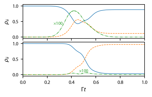
Plot up the state populations \(\rho_{gg}\) (blue), \(\rho_{rr}\) (orange), and \(\rho_{ee}\) (green) vs. time. We see that STIRAP is only effective in the correct order (solid), and it maintains a minium of population in \(|e\rangle>\). The incorrect order (dashed) is nearly completely ineffective at state transfer.
[4]:
fig, ax = plt.subplots(2, 1, figsize=(3.25, 2.))
factors = [1, 1, 1e2]
linespecs = ['-', '--', '-.']
for ii, factor in enumerate(factors):
    ax[0].plot(sol1.t/1e3, factor*np.real(sol1.rho[ii, ii]),
               linespecs[ii], color='C%d'%ii, linewidth=0.75)
    ax[1].plot(sol2.t/1e3, factor*np.real(sol2.rho[ii, ii]),
               linespecs[ii], color='C%d'%ii, linewidth=0.75)

[ax[ii].set_ylabel('$\\rho_{ii}$') for ii in range (2)];
[ax[ii].set_xlim((0, 1)) for ii in range(2)];
ax[1].set_xlabel('$\Gamma t$')
ax[0].xaxis.set_ticklabels('')
ax[0].text(0.25, 0.4,'$\\times100$',fontsize=7, color='C2')
ax[1].text(0.46, 0.075,'$\\times100$',fontsize=7, color='C2')
fig.subplots_adjust(bottom=0.18, left=0.14)