\(F=0 \rightarrow F'=1\) MOT forces with the OBEs
This example covers calculating the forces in a one-dimensional MOT using the optical bloch equations. This example does the boring thing and checks that everything is working on the \(F=0 \rightarrow F'=1\) transition.
It first checks the force along the \(\hat{z}\)-direction. One should look to see that things agree with what one expects whether or not one puts the detuning on the lasers or on the Hamilonian. One should also look at whether the force depends on transforming the OBEs into the real/imaginary components.
It then checks the force along the \(\hat{x}\) and \(\hat{y}\) directions. This is important because the OBEs solve this in a different way compared to the rate equations. Whereas the rate equatons rediagonalize the Hamiltonian for a given direction, the OBE solves everything in the \(\hat{z}\)-basis.
Finally, we plop an atom into the 1D MOT and see how it evolves with time.
[1]:
import numpy as np
import matplotlib.pyplot as plt
import pylcp
import time
Define the problem
We will define multiple laser beam configurations to start, namely with beams pointed along each axis. Of course, we must also define the Hamiltonian and magnetic field.
[2]:
laser_det = 0
ham_det = -2.5
s = 1.
transform = True

laserBeams = {}
laserBeams['x'] = pylcp.laserBeams([
    {'kvec':np.array([ 1., 0., 0.]), 'pol':-1, 'delta':laser_det, 's':s},
    {'kvec':np.array([-1., 0., 0.]), 'pol':-1, 'delta':laser_det, 's':s},
    ], beam_type=pylcp.infinitePlaneWaveBeam)
laserBeams['y'] = pylcp.laserBeams([
    {'kvec':np.array([0.,  1., 0.]), 'pol':-1, 'delta':laser_det, 's':s},
    {'kvec':np.array([0., -1., 0.]), 'pol':-1, 'delta':laser_det, 's':s}
    ], beam_type=pylcp.infinitePlaneWaveBeam)
laserBeams['z'] = pylcp.laserBeams([
    {'kvec':np.array([0., 0.,  1.]), 'pol':+1, 'delta':laser_det, 's':s},
    {'kvec':np.array([0., 0., -1.]), 'pol':+1, 'delta':laser_det, 's':s}
    ], beam_type=pylcp.infinitePlaneWaveBeam)

alpha = 1e-3
magField = pylcp.quadrupoleMagneticField(alpha)

# Hamiltonian for F=0->F=1
H_g, muq_g = pylcp.hamiltonians.singleF(F=0, gF=0, muB=1)
H_e, muq_e = pylcp.hamiltonians.singleF(F=1, gF=1, muB=1)
d_q = pylcp.hamiltonians.dqij_two_bare_hyperfine(0, 1)
hamiltonian = pylcp.hamiltonian(H_g, H_e - ham_det*np.eye(3), muq_g, muq_e, d_q, mass=250)
Compute equilibrium force along \(\hat{z}\)
This checks to make sure that the rate equations and OBE agree:
[3]:
obe={}
rateeq={}

obe['z'] = {}
rateeq['z'] = {}

z = np.arange(-5.0, 5.01, 0.25)

rateeq['z'] = pylcp.rateeq(laserBeams['z'], magField, hamiltonian)
rateeq['z'].generate_force_profile(
    [np.zeros(z.shape), np.zeros(z.shape), z/alpha],
    np.zeros((3,) + z.shape),
    name='MOT_1'
)

obe['z'] = pylcp.obe(laserBeams['z'], magField, hamiltonian,
                     transform_into_re_im=transform,
                     include_mag_forces=True)
obe['z'].generate_force_profile(
    [np.zeros(z.shape), np.zeros(z.shape), z/alpha],
    np.zeros((3,) + z.shape),
    name='MOT_1', deltat_tmax=2*np.pi*100, deltat_r=4/alpha,
    itermax=1000, progress_bar=True
);
Completed in 7.75 s.
Plot up the results:
[4]:
fig, ax = plt.subplots(3, 2, num='Optical Molasses F=0->F1', figsize=(6.5, 3*2.25))

Es = np.zeros((z.size, 4))
for ii, z_i in enumerate(z):
    Bq = np.array([0., magField.Field(np.array([0., 0., z_i/alpha]))[2], 0])
    Es[ii, :] = np.real(np.diag(hamiltonian.return_full_H({'g->e':np.array([0., 0., 0.])}, Bq)))

[ax[0, 0].plot(z, Es[:, 1+jj], label='$m_F=%d$'%(jj-1)) for jj in range(3)]
ax[0, 0].legend(fontsize=6)
ax[0, 0].set_ylabel('$E/(\hbar \Gamma)$')

types = ['-', '--', '-.']
lbls = ['+k','-k']
ax[0, 1].plot(obe['z'].profile['MOT_1'].R[2]*alpha,
           obe['z'].profile['MOT_1'].F[2],
           label='OBE', linewidth=0.75)
ax[0, 1].plot(rateeq['z'].profile['MOT_1'].R[2]*alpha,
           rateeq['z'].profile['MOT_1'].F[2],
           label='Rate Eq.', linewidth=0.5)
for jj in range(2):
    ax[0, 1].plot(obe['z'].profile['MOT_1'].R[2]*alpha,
                  obe['z'].profile['MOT_1'].f['g->e'][2, :, jj],
                  types[jj+1], color='C0', linewidth=0.75, label=lbls[jj])
    ax[0, 1].plot(rateeq['z'].profile['MOT_1'].R[2]*alpha,
                  rateeq['z'].profile['MOT_1'].f['g->e'][2, :, jj],
                  types[jj+1], color='C1', linewidth=0.5)
ax[0, 1].legend(fontsize=6)
ax[0, 1].set_ylabel('$f/(\hbar k \Gamma)$')

for q in range(3):
    ax[1, 1].plot(z, obe['z'].profile['MOT_1'].fq['g->e'][2, :, q, 0], types[q],
            linewidth=0.5, color='C0', label='$+k$, $q=%d$'%(q-1))
    ax[1, 1].plot(z, obe['z'].profile['MOT_1'].fq['g->e'][2, :, q, 1], types[q],
            linewidth=0.5, color='C1', label='$-k$, $q=%d$'%(q-1))
ax[1, 1].plot(z, obe['z'].profile['MOT_1'].F[2], 'k-',
           linewidth=0.75)
ax[1, 1].legend(fontsize=6)
ax[1, 1].set_xlabel('$z/(\mu_B \hbar B\'/\Gamma)$')
ax[1, 1].set_ylabel('$f/(\hbar k \Gamma)$')
fig.subplots_adjust(wspace=0.15)

ax[1, 0].plot(z, rateeq['z'].profile['MOT_1'].Neq[:, 0], '--',
              linewidth=0.75, label='$F=0$ (RE)')
ax[1, 0].plot(z, obe['z'].profile['MOT_1'].Neq[:, 0], '-',
              linewidth=0.5, color='C0', label='$F=0$ (OBE)')
for jj in range(3):
    ind = z<=0
    ax[1, 0].plot(z[ind], rateeq['z'].profile['MOT_1'].Neq[ind, 3-jj], '--',
                  linewidth=0.75, color='C%d'%jj, label='$m_F=%d$'%(jj-1))
    ind = z>=0
    ax[1, 0].plot(z[ind], rateeq['z'].profile['MOT_1'].Neq[ind, jj+1], '--',
                  linewidth=0.75, color='C%d'%jj)
    ax[1, 0].plot(z, obe['z'].profile['MOT_1'].Neq[:, jj+1], '-',
                  linewidth=0.5, color='C%d'%jj)

ax[1, 0].legend(fontsize=6)
ax[1, 0].set_ylabel('$N_{eq}$')

ax[2, 0].plot(z, 1e5*obe['z'].profile['MOT_1'].f_mag[2], linewidth=0.75)
ax[2, 0].plot(z, 1e5*rateeq['z'].profile['MOT_1'].f_mag[2], linewidth=0.5)
ax[2, 0].set_ylabel('$10^5 f_{\\rm mag}/\hbar k \Gamma$')
ax[2, 0].set_xlabel('$z/(\mu_B \hbar B\'/\Gamma)$')
ax[2, 1].set_xlabel('$z/(\mu_B \hbar B\'/\Gamma)$')
fig.subplots_adjust(left=0.08, wspace=0.25)
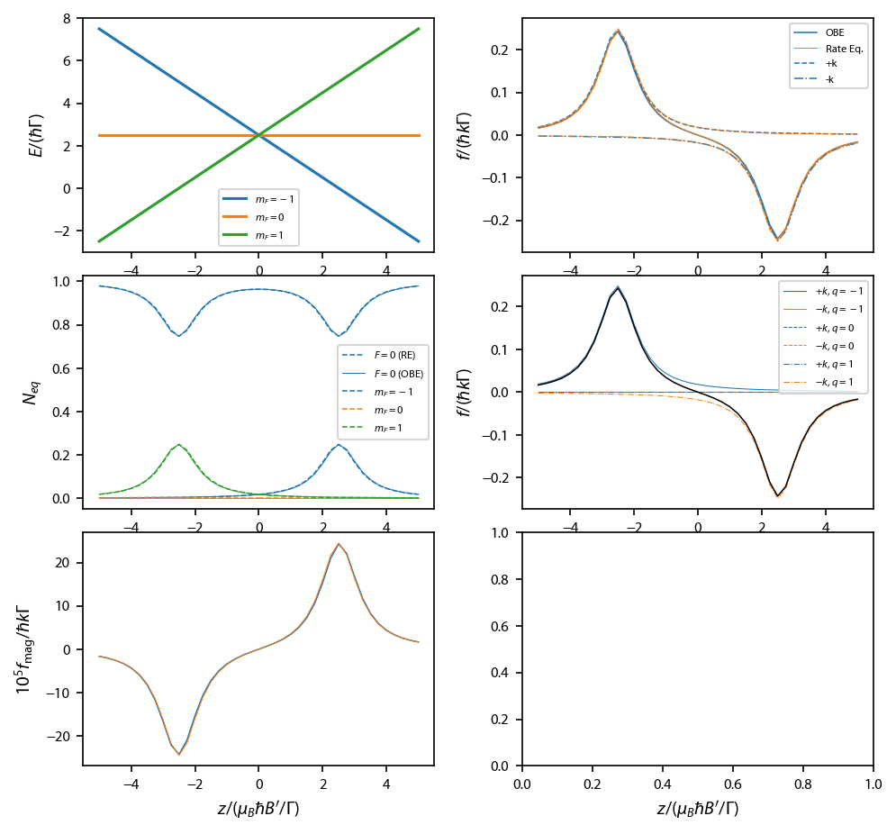
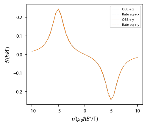
Compute equilibrium forces along \(\hat{x}\) and \(\hat{y}\)
Same as before, this steps makes sure that the OBEs are correctly evolving in other directions.
[5]:
R = {}
R['x'] = [2*z/alpha, np.zeros(z.shape), np.zeros(z.shape)]
R['y'] = [np.zeros(z.shape), 2*z/alpha, np.zeros(z.shape)]

for key in ['x','y']:
    rateeq[key] = pylcp.rateeq(laserBeams[key], magField,
                               hamiltonian)
    rateeq[key].generate_force_profile(
        R[key], np.zeros((3,) + z.shape), name='MOT_1'
    )

    obe[key] = pylcp.obe(laserBeams[key], magField,  hamiltonian,
                         transform_into_re_im=transform,
                         include_mag_forces=False)

    obe[key].generate_force_profile(
        R[key], np.zeros((3,) + z.shape), name='MOT_1',
        deltat_tmax=2*np.pi*100, deltat_r=4/alpha, itermax=1000,
        progress_bar=True,
    )
Completed in 6.66 s.
Completed in 6.48 s.
Plot this one up:
[6]:
fig, ax = plt.subplots(1, 1)
for ii, key in enumerate(['x','y']):
    ax.plot(obe[key].profile['MOT_1'].R[ii]*alpha,
            obe[key].profile['MOT_1'].F[ii],
            label='OBE + %s' % key, color='C%d'%ii, linewidth=0.5)
    ax.plot(rateeq[key].profile['MOT_1'].R[ii]*alpha,
            rateeq[key].profile['MOT_1'].F[ii], '--',
            label='Rate eq + %s' % key, color='C%d'%ii, linewidth=0.5)
ax.legend(fontsize=6)
ax.set_xlabel('$r/(\mu_B \hbar B\'/\Gamma)$')
ax.set_ylabel('$f/(\hbar k \Gamma)$');
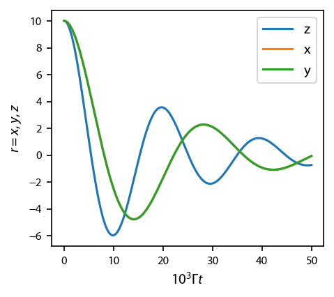
Place an atom in this MOT
We’ll place it at rest, but displaced from the origin. It should first be accelerated toward the origin then damped. Depending on the mass parameter, it may execute an oscillation or two.
[7]:
for key in obe:
    if key is 'x':
        ii = 0
    elif key is 'y':
        ii = 1
    elif key is 'z':
        ii = 2

    r0 = np.zeros((3,))
    r0[ii] = 10.

    obe[key].set_initial_position(r0)
    obe[key].set_initial_velocity(np.zeros((3,)))
    obe[key].set_initial_rho_from_rateeq()

    freeze_axis = [True]*3
    freeze_axis[ii] = False

    obe[key].evolve_motion([0, 5e4],
                           freeze_axis=freeze_axis,
                           progress_bar=True,
                           random_recoil=False
                          )
Completed in 2:06.
Completed in 1:42.
Completed in 1:41.
[9]:
fig, ax = plt.subplots(1, 1)
for key in obe:
    if key is 'x':
        ii = 0
    elif key is 'y':
        ii = 1
    elif key is 'z':
        ii = 2

    ax.plot(obe[key].sol.t/1e3, obe[key].sol.r[ii], label=key)

ax.legend()
ax.set_xlabel('$10^3 \Gamma t$')
ax.set_ylabel('$r=x,y,z$');