Real atoms in a MOT
This example covers calculating the forces in various type-I and type-II three-dimensional MOT with real atoms and comparing the results.
[1]:
import numpy as np
import matplotlib.pyplot as plt
import scipy.constants as cts
import pylcp
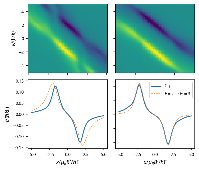
\(^7\)Li: compare the D\(_2\) line with a basic \(F=2\rightarrow F=3\) transition
We’ll do this specifically for \(^7\)Li. As usual, we first define the Hamiltonian, laser Beams, and magnetic field. We start with the full D\(_2\) line. Note that we need to specify a repump laser, which, for \(^7\)Li, generally has the same red detuning as the main cooling beam.
[2]:
det = -2.0
alpha = 1.0
s = 1.0

# Define the atomic Hamiltonian for 7Li:
atom = pylcp.atom("7Li")
H_g_D2, mu_q_g_D2 = pylcp.hamiltonians.hyperfine_coupled(
    atom.state[0].J, atom.I, atom.state[0].gJ, atom.gI,
    atom.state[0].Ahfs/atom.state[2].gammaHz, Bhfs=0, Chfs=0,
    muB=1)
H_e_D2, mu_q_e_D2 = pylcp.hamiltonians.hyperfine_coupled(
    atom.state[2].J, atom.I, atom.state[2].gJ, atom.gI,
    Ahfs=atom.state[2].Ahfs/atom.state[2].gammaHz,
    Bhfs=atom.state[2].Bhfs/atom.state[2].gammaHz, Chfs=0,
    muB=1)

dijq_D2 = pylcp.hamiltonians.dqij_two_hyperfine_manifolds(
    atom.state[0].J, atom.state[2].J, atom.I)

E_e_D2 = np.unique(np.diagonal(H_e_D2))
E_g_D2 = np.unique(np.diagonal(H_g_D2))

hamiltonian_D2 = pylcp.hamiltonian(H_g_D2, H_e_D2, mu_q_g_D2, mu_q_e_D2, dijq_D2)

# Now, we need to sets of laser beams -> one for F=1->2 and one for F=2->3:
laserBeams_cooling_D2 = pylcp.conventional3DMOTBeams(
    s=s, delta=(E_e_D2[0] - E_g_D2[1]) + det)
laserBeams_repump_D2 = pylcp.conventional3DMOTBeams(
    s=s, delta=(E_e_D2[1] - E_g_D2[0]) + det)
laserBeams_D2 = laserBeams_cooling_D2 + laserBeams_repump_D2

magField = pylcp.quadrupoleMagneticField(alpha)
Construct the rate equations for the full D\(_2\) line and calculate a force profile:
[3]:
x = np.arange(-5, 5.1, 0.2)
v = np.arange(-5, 5.1, 0.2)

dx = np.mean(np.diff(x))
dv = np.mean(np.diff(v))

X, V = np.meshgrid(x, v)

# Define the trap:
trap_D2 = pylcp.rateeq(
    laserBeams_D2, magField, hamiltonian_D2,
    include_mag_forces=False
)
trap_D2.generate_force_profile(
    [np.zeros(X.shape), np.zeros(X.shape), X],
    [np.zeros(V.shape), np.zeros(V.shape), V],
    name='Fz')
FzLi_D2 = trap_D2.profile['Fz'].F[2]
Now, repeat the same procedure for the simpler \(F=2\rightarrow F'=3\) transition, making sure we keep the g-factors the same:
[4]:
# Define the atomic Hamiltonian for F-> 2 to 3:
H_g_23, mu_q_g_23 = pylcp.hamiltonians.singleF(F=2, gF=1/2, muB=1)
H_e_23, mu_q_e_23 = pylcp.hamiltonians.singleF(F=3, gF=2/3, muB=1)

dijq_23 = pylcp.hamiltonians.dqij_two_bare_hyperfine(2, 3)

hamiltonian_23 = pylcp.hamiltonian(H_g_23, H_e_23, mu_q_g_23, mu_q_e_23, dijq_23)

# Define the laser beams for 2->3
laserBeams_23 = pylcp.conventional3DMOTBeams(s=s, delta=det)

# Make the trap for 2->3
trap_23 = pylcp.rateeq(
    laserBeams_23, magField, hamiltonian_23, include_mag_forces=False)
trap_23.generate_force_profile(
    [np.zeros(X.shape), np.zeros(X.shape), X],
    [np.zeros(V.shape), np.zeros(V.shape), V],
    name='Fz')
Fz2to3 = trap_23.profile['Fz'].F[2]
Plot up the results:
[5]:
fig, ax = plt.subplots(2, 2, figsize=(1.5*3.25, 1.5*2.75))
ax[0, 0].imshow(FzLi_D2, origin='bottom',
               extent=(np.amin(x)-dx/2, np.amax(x)+dx/2,
                       np.amin(v)-dv/2, np.amax(v)+dv/2),
               aspect='auto')
ax[0, 1].imshow(Fz2to3, origin='bottom',
               extent=(np.amin(x)-dx/2, np.amax(x)+dx/2,
                       np.amin(v)-dv/2, np.amax(v)+dv/2),
               aspect='auto')
ax[1, 0].plot(X[int(X.shape[0]/2), :],
              FzLi_D2[int(X.shape[0]/2), :])
ax[1, 0].plot(X[int(X.shape[0]/2), :],
              Fz2to3[int(X.shape[0]/2), :], '--',
              linewidth=0.75)
ax[1, 1].plot(V[:, int(X.shape[1]/2)+1],
              FzLi_D2[:, int(X.shape[1]/2)+1], label='$^7$Li')
ax[1, 1].plot(V[:, int(X.shape[1]/2)+1],
              Fz2to3[:, int(X.shape[1]/2)+1], '--',
              label='$F=2 \\rightarrow F\'=3$',
              linewidth=0.75)

ax[1, 1].legend(fontsize=8)

[ax[ii, 1].yaxis.set_ticklabels('') for ii in range(2)]
[ax[0, ii].xaxis.set_ticklabels('') for ii in range(2)]

ax[0, 0].set_ylabel('$v/(\Gamma/k)$')
ax[1, 0].set_ylabel('$f/(\hbar k \Gamma)$')
ax[1, 0].set_xlabel('$x/\mu_B B\'/\hbar\Gamma$')
ax[1, 1].set_xlabel('$x/\mu_B B\'/\hbar\Gamma$');

Now, it seems to me that because of the un-resolved hyperfine structure in the excited state that is inherent in 7Li, the repump, which drives \(F=1\rightarrow F'=2\) transitions will also contribute the trapping and cause most of the difference between the \(F=2\rightarrow F=3\) and the full Hamiltonian calculation.
Switch to \(^{87}\)Rb
By switching to 87Rb we can bring the repump to resonance, and turn down its intensity to 1/100 of the main cooling light.
[6]:
atom = pylcp.atom("87Rb")
H_g_D2, mu_q_g_D2 = pylcp.hamiltonians.hyperfine_coupled(
    atom.state[0].J, atom.I, atom.state[0].gJ, atom.gI,
    atom.state[0].Ahfs/atom.state[2].gammaHz, Bhfs=0, Chfs=0,
    muB=1)
H_e_D2, mu_q_e_D2 = pylcp.hamiltonians.hyperfine_coupled(
    atom.state[2].J, atom.I, atom.state[2].gJ, atom.gI,
    Ahfs=atom.state[2].Ahfs/atom.state[2].gammaHz,
    Bhfs=atom.state[2].Bhfs/atom.state[2].gammaHz, Chfs=0,
    muB=1)
mu_q_g_D2[1]
dijq_D2 = pylcp.hamiltonians.dqij_two_hyperfine_manifolds(
    atom.state[0].J, atom.state[2].J, atom.I)

E_e_D2 = np.unique(np.diagonal(H_e_D2))
E_g_D2 = np.unique(np.diagonal(H_g_D2))

hamiltonian_D2 = pylcp.hamiltonian(H_g_D2, H_e_D2, mu_q_g_D2, mu_q_e_D2, dijq_D2)

# Now, we need to sets of laser beams -> one for F=1->2 and one for F=2->3:
laserBeams_cooling_D2 = pylcp.conventional3DMOTBeams(
    s=s, delta=(E_e_D2[-1] - E_g_D2[-1]) + det)
laserBeams_repump_D2 = pylcp.conventional3DMOTBeams(
    s=0.01*s, delta=(E_e_D2[-2] - E_g_D2[-2]))
laserBeams_D2 = laserBeams_cooling_D2 + laserBeams_repump_D2
Construct the full rate equations for the D\(_2\) line:
[7]:
trap_D2 = pylcp.rateeq(
    laserBeams_D2, magField, hamiltonian_D2, include_mag_forces=False)
trap_D2.generate_force_profile(
    [np.zeros(X.shape), np.zeros(X.shape), X],
    [np.zeros(V.shape), np.zeros(V.shape), V],
    name='Fz')
FzRb_D2 = trap_D2.profile['Fz'].F[2]
Plot up the results:
[8]:
fig, ax = plt.subplots(2, 2, figsize=(1.5*3.25, 1.5*2.75))
ax[0, 0].imshow(FzLi_D2, origin='bottom',
               extent=(np.amin(x)-dx/2, np.amax(x)+dx/2,
                       np.amin(v)-dv/2, np.amax(v)+dv/2),
               aspect='auto')
ax[0, 1].imshow(Fz2to3, origin='bottom',
               extent=(np.amin(x)-dx/2, np.amax(x)+dx/2,
                       np.amin(v)-dv/2, np.amax(v)+dv/2),
               aspect='auto')
ax[1, 0].plot(X[int(X.shape[0]/2), :],
              FzLi_D2[int(X.shape[0]/2), :])
ax[1, 0].plot(X[int(X.shape[0]/2), :],
              Fz2to3[int(X.shape[0]/2), :], '--',
              linewidth=0.75)
ax[1, 1].plot(V[:, int(X.shape[1]/2)+1],
              FzLi_D2[:, int(X.shape[1]/2)+1], label='$^7$Li')
ax[1, 1].plot(V[:, int(X.shape[1]/2)+1],
              Fz2to3[:, int(X.shape[1]/2)+1], '--',
              label='$F=2 \\rightarrow F\'=3$',
              linewidth=0.75)

ax[1, 1].legend(fontsize=8)

[ax[ii, 1].yaxis.set_ticklabels('') for ii in range(2)]
[ax[0, ii].xaxis.set_ticklabels('') for ii in range(2)]

ax[0, 0].set_ylabel('$v/(\Gamma/k)$')
ax[1, 0].set_ylabel('$f/(\hbar k \Gamma)$')
ax[1, 0].set_xlabel('$x/\mu_B B\'/\hbar\Gamma$')
ax[1, 1].set_xlabel('$x/\mu_B B\'/\hbar\Gamma$');
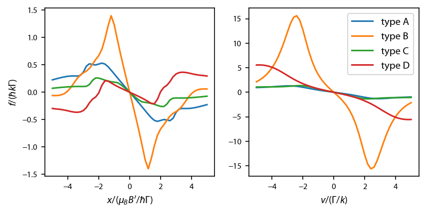
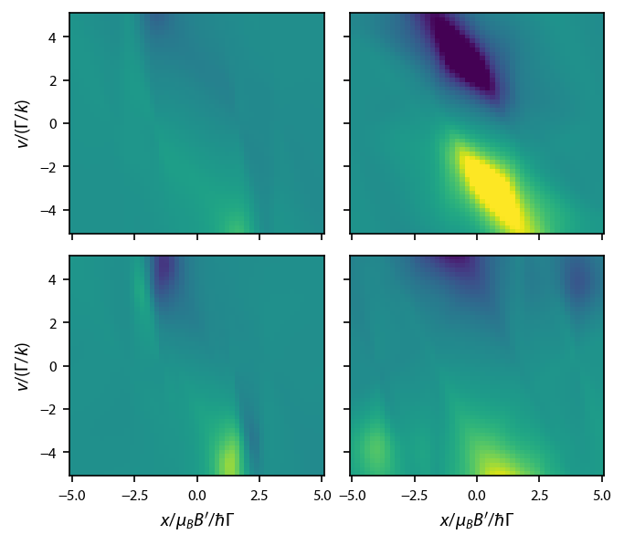
\(^{23}\)Na: type-I MOTs
Now let’s cover the four type I (type-I/type-II) MOTs of J. Flemming, et. al., Opt. Commun. 135, 269 (1997). We must loop through the four types.
[9]:
atom = pylcp.atom("23Na")
H_g_D1, Bq_g_D1 = pylcp.hamiltonians.hyperfine_coupled(
    atom.state[0].J, atom.I, atom.state[0].gJ, atom.gI,
    atom.state[0].Ahfs/atom.state[1].gammaHz, Bhfs=0, Chfs=0,
    muB=3)
H_e_D1, Bq_e_D1 = pylcp.hamiltonians.hyperfine_coupled(
    atom.state[1].J, atom.I, atom.state[1].gJ, atom.gI,
    Ahfs=atom.state[1].Ahfs/atom.state[1].gammaHz,
    Bhfs=atom.state[1].Bhfs/atom.state[1].gammaHz, Chfs=0,
    muB=3)

E_g_D1 = np.unique(np.diagonal(H_g_D1))
E_e_D1 = np.unique(np.diagonal(H_e_D1))

dijq_D1 = pylcp.hamiltonians.dqij_two_hyperfine_manifolds(
    atom.state[0].J, atom.state[1].J, atom.I)

hamiltonian_D1 = pylcp.hamiltonian(H_g_D1, H_e_D1, Bq_g_D1, Bq_e_D1, dijq_D1)

# Conditions taken from the paper, Table 1:
conds = np.array([[1, 1, -25/10, -1, 2, 1, -60/10, +1],
                  [1, 1, -20/10, -1, 2, 2, -30/10, +1],
                  [1, 2, -20/10, +1, 2, 1, -50/10, +1],
                  [1, 2, -40/10, +1, 2, 2, -60/10, +1]])

FzNa_D1 = np.zeros((4,) + FzRb_D2.shape)
for ii, cond in enumerate(conds):
    laserBeams_laser1 = pylcp.conventional3DMOTBeams(
        s=s, delta=(E_e_D1[int(cond[1]-1)] - E_g_D1[0]) + cond[2], pol=cond[3])
    laserBeams_laser2 = pylcp.conventional3DMOTBeams(
        s=s, delta=(E_e_D1[int(cond[5]-1)] - E_g_D1[1]) + cond[6], pol=cond[7])
    laserBeams_D1 = laserBeams_laser1 + laserBeams_laser2

    # Calculate the forces:
    trap_D1 = pylcp.rateeq(
        laserBeams_D1, magField, hamiltonian_D1, include_mag_forces=False)
    trap_D1.generate_force_profile(
        [np.zeros(X.shape), np.zeros(X.shape), X],
        [np.zeros(V.shape), np.zeros(V.shape), V],
        name='Fz')
    FzNa_D1[ii] = trap_D1.profile['Fz'].F[2]
Plot up the force vs. classical phase space:
[10]:
lim = np.amax(np.abs(FzNa_D1))
fig, ax = plt.subplots(2, 2, figsize=(1.5*3.25, 1.5*2.75))
ax[0, 0].imshow(FzNa_D1[0], origin='bottom',
                extent=(np.amin(x)-dx/2, np.amax(x)+dx/2,
                        np.amin(v)-dv/2, np.amax(v)+dv/2),
                aspect='auto', clim=(-0.01, 0.01))
ax[0, 1].imshow(FzNa_D1[1], origin='bottom',
                extent=(np.amin(x)-dx/2, np.amax(x)+dx/2,
                        np.amin(v)-dv/2, np.amax(v)+dv/2),
                aspect='auto', clim=(-0.01, 0.01))
ax[1, 0].imshow(FzNa_D1[2], origin='bottom',
                extent=(np.amin(x)-dx/2, np.amax(x)+dx/2,
                        np.amin(v)-dv/2, np.amax(v)+dv/2),
                aspect='auto', clim=(-0.01, 0.01))
ax[1, 1].imshow(FzNa_D1[3], origin='bottom',
                extent=(np.amin(x)-dx/2, np.amax(x)+dx/2,
                        np.amin(v)-dv/2, np.amax(v)+dv/2),
                aspect='auto', clim=(-0.01, 0.01))

[ax[ii, 1].yaxis.set_ticklabels('') for ii in range(2)]
[ax[0, ii].xaxis.set_ticklabels('') for ii in range(2)]

ax[0, 0].set_ylabel('$v/(\Gamma/k)$')
ax[1, 0].set_ylabel('$v/(\Gamma/k)$')
ax[1, 0].set_xlabel('$x/\mu_B B\'/\hbar\Gamma$')
ax[1, 1].set_xlabel('$x/\mu_B B\'/\hbar\Gamma$');
[16]:
fig, ax = plt.subplots(1, 2, figsize=(6.25, 2.75))
types = ['A','B','C','D']
for ii in range(4):
    ax[0].plot(x, 1e3*FzNa_D1[ii][int(len(x)/2),:], label='type ' + types[ii])
    ax[1].plot(v, 1e3*FzNa_D1[ii][:,int(len(v)/2)], label='type ' + types[ii])
ax[1].legend()
ax[0].set_xlabel('$x/(\mu_B B\'/\hbar \Gamma)$')
ax[1].set_xlabel('$v/(\Gamma/k)$')
ax[0].set_ylabel('$f/(\hbar k \Gamma)$')
fig.subplots_adjust(wspace=0.2)