Recoil-limited MOT

In this example, we simulate a recoil-limited MOT like the Sr red MOT. Let’s use the bosonic isotope, which is a \(F=0\rightarrow F'=1\) transition. In this case, we can use heuristiceq along with either obe or rateeq. Our results can be compared to R.K. Hanley, P. Huillery, N.C. Keegan, A.D. Bounds, D. Boddy, R. Faoro, and M.P.A. Jones, “Quantitative simulation of a magneto-optical trap operating near the photon recoil limit” Journal of Modern Optics 65, 667 (2018). https://dx.doi.org/10.1080/09500340.2017.1401679

import numpy as np
import matplotlib.pyplot as plt
import pylcp
import scipy.constants as cts
from pylcp.common import progressBar

Let’s develop a unit system appropriate for \(^{88}\)Sr:

k = 2*np.pi/689E-7    # cm^{-1}
x0 = 1/k              # our length scale in cm
gamma = 2*np.pi*7.5e3 # 7.5 kHz linewidth
t0 = 1/gamma          # our time scale in s

# Magnetic field gradient parameter (the factor of 3/2 comes from the
# excited state g-factor.)
alpha = (3/2)*cts.value('Bohr magneton in Hz/T')*1e-4*8*x0/7.5E3

# The unitless mass parameter:
mass = 87.8*cts.value('atomic mass constant')*(x0*1e-2)**2/cts.hbar/t0

# Gravity
g = -np.array([0., 0., 9.8*t0**2/(x0*1e-2)])

print(x0, t0, mass, alpha, g)

1.0965775579031588e-05 2.1220659078919377e-05 0.7834067174281623 0.02455674894694879 [-0.         -0.         -0.04024431]

Now define the problem:

We define a preliminary detuning, intensity, along with the basic Hamiltonian, laser beams, and magnetic field:

s = 25
det = -200/7.5

magField = pylcp.quadrupoleMagneticField(alpha)

laserBeams = pylcp.conventional3DMOTBeams(delta=det, s=s,
                                          beam_type=pylcp.infinitePlaneWaveBeam)

Hg, mugq = pylcp.hamiltonians.singleF(F=0, muB=1)
He, mueq = pylcp.hamiltonians.singleF(F=1, muB=1)

dq = pylcp.hamiltonians.dqij_two_bare_hyperfine(0, 1)

hamiltonian = pylcp.hamiltonian(Hg, He, mugq, mueq, dq, mass=mass)

#eqn = pylcp.heuristiceq(laserBeams, magField, g, mass=mass)
eqn = pylcp.rateeq(laserBeams, magField, hamiltonian, g)

Generate a force profile:

We can compare this to Fig. 1 of the reference above.

z = np.linspace(-0.2, 0.2, 101)/(10*x0)

R = np.array([np.zeros(z.shape), np.zeros(z.shape), z])
V = np.zeros((3,) + z.shape)

eqn.generate_force_profile(R, V, name='Fz')

fig, ax = plt.subplots(1, 1)

ax.plot(z*(10*x0), eqn.profile['Fz'].F[2])
ax.set_xlabel('$z$ (mm)')
ax.set_ylabel('$f/(\hbar k \Gamma)$');

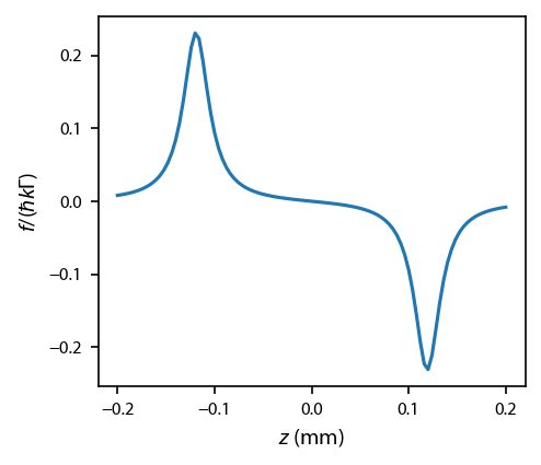
Note in the paper they have the \(F\) in units of N. When adding the \(\hbar k \Gamma\) to mine, I find my force is a factor of 2 lower than theirs in the plot.

Dynamics

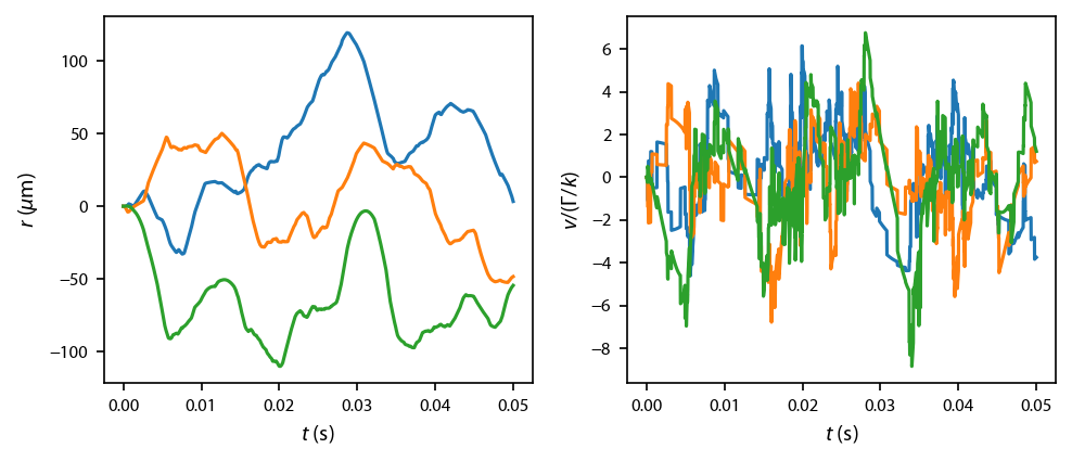
Before we run hundreds of simultions, let’s first run a single simulation of an atom just to make sure that everything is working:

tmax = 0.05/t0
if isinstance(eqn, pylcp.rateeq):
    eqn.set_initial_pop(np.array([1., 0., 0., 0.]))
eqn.set_initial_position(np.array([0., 0., 0.]))
eqn.evolve_motion([0, 0.05/t0], random_recoil=True, progress_bar=True, max_step=1.)

Completed in 18.50 s.

Plot up this test solution:

fig, ax = plt.subplots(1, 2, figsize=(6.5, 2.75))
ax[0].plot(eqn.sol.t*t0, eqn.sol.r.T*(1e4*x0))
ax[1].plot(eqn.sol.t*t0, eqn.sol.v.T)
ax[0].set_ylabel('$r$ ($\mu$m)')
ax[0].set_xlabel('$t$ (s)')
ax[1].set_ylabel('$v/(\Gamma/k)$')
ax[1].set_xlabel('$t$ (s)')
fig.subplots_adjust(left=0.08, wspace=0.22)

Now simulate many atoms

Here, we use the pathos package to do parallel processing

import pathos

if hasattr(eqn, 'sol'):
    del eqn.sol

def generate_random_solution(x, eqn=eqn, tmax=tmax):
    # We need to generate random numbers to prevent solutions from being seeded
    # with the same random number.
    import numpy as np

    np.random.rand(256*x)
    eqn.evolve_motion(
        [0, tmax],
        t_eval=np.linspace(0, tmax, 1001),
        random_recoil=True,
        progress_bar=False,
        max_step=1.
    )

    return eqn.sol

Natoms = 1024
chunksize = 4
sols = []
progress = progressBar()
for jj in range(int(Natoms/chunksize)):
    with pathos.pools.ProcessPool(nodes=4) as pool:
        sols += pool.map(generate_random_solution, range(chunksize))
    progress.update((jj+1)/(Natoms/chunksize))

Completed in 1:33:54.

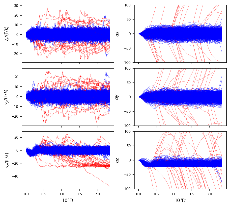
Plot up all the trajectories. We make a basic ejected criterion, which says that if the atom flies more than 500 \(\mu\)m away from the origin in either \(\hat{x}\) or \(\hat{y}\), we say that atom is ejected:

ejected = [np.bitwise_or(
    np.abs(sol.r[0, -1]*(1e4*x0))>500,
    np.abs(sol.r[1, -1]*(1e4*x0))>500
) for sol in sols]

print('Number of ejected atoms: %d' % np.sum(ejected))
fig, ax = plt.subplots(3, 2, figsize=(6.25, 2*2.75))
for sol, ejected_i in zip(sols, ejected):
    for ii in range(3):
        if ejected_i:
            ax[ii, 0].plot(sol.t/1e3, sol.v[ii], color='r', linewidth=0.25)
            ax[ii, 1].plot(sol.t/1e3, sol.r[ii]*alpha, color='r', linewidth=0.25)
        else:
            ax[ii, 0].plot(sol.t/1e3, sol.v[ii], color='b', linewidth=0.25)
            ax[ii, 1].plot(sol.t/1e3, sol.r[ii]*alpha, color='b', linewidth=0.25)

"""for ax_i in ax[:, 0]:
    ax_i.set_ylim((-0.75, 0.75))
for ax_i in ax[:, 1]:
    ax_i.set_ylim((-4., 4.))"""
for ax_i in ax[-1, :]:
    ax_i.set_xlabel('$10^3 \Gamma t$')
for jj in range(2):
    for ax_i in ax[jj, :]:
        ax_i.set_xticklabels('')
for ax_i, lbl in zip(ax[:, 0], ['x','y','z']):
    ax_i.set_ylabel('$v_' + lbl + '/(\Gamma/k)$')
for ax_i, lbl in zip(ax[:, 1], ['x','y','z']):
    ax_i.set_ylim((-100, 100))
    ax_i.set_ylabel('$\\alpha ' + lbl + '$')

fig.subplots_adjust(left=0.1, bottom=0.08, wspace=0.22)

Number of ejected atoms: 39

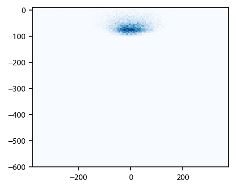
Now, every 0.1 ms, bin the \(x\) and \(z\) coordinates, make a histogram, and simulate an image:

allx = np.array([], dtype='float64')
allz = np.array([], dtype='float64')

for sol in sols:
    allx = np.append(allx, sol.r[0][200::100]*(1e4*x0))
    allz = np.append(allz, sol.r[2][200::100]*(1e4*x0))

img, x_edges, z_edges = np.histogram2d(allx, allz, bins=[np.arange(-375, 376, 5.), np.arange(-600., 11., 5.)])

fig, ax = plt.subplots(1, 1)
im = ax.imshow(img.T, origin='bottom',
               extent=(np.amin(x_edges), np.amax(x_edges),
                       np.amin(z_edges), np.amax(z_edges)),
               cmap='Blues',
               aspect='equal')

Now, let’s run the detuning

And produce the resulting simulated MOT images

dets = np.array([det, -400/7.5, -600/7.5, -800/7.5])
#s = 9

imgs = np.zeros(dets.shape + img.shape)
num_of_ejections = np.zeros(dets.shape)
num_of_ejections[0] = np.sum(ejected)
imgs[0] = img

for ii, det in enumerate(dets[1:]):
    # Rewrite the laser beams with the new detuning
    laserBeams = pylcp.conventional3DMOTBeams(delta=det, s=s,
                                              beam_type=pylcp.infinitePlaneWaveBeam)

    # Make the equation:
    eqn = pylcp.rateeq(laserBeams, magField, hamiltonian, g)
    if isinstance(eqn, pylcp.rateeq):
        eqn.set_initial_pop(np.array([1., 0., 0., 0.]))

    # Use the last equilibrium position to set this position:
    eqn.set_initial_position(np.array([0., 0., np.mean(allz)]))

    # Re-define the random soluton:
    def generate_random_solution(x, eqn=eqn, tmax=tmax):
        # We need to generate random numbers to prevent solutions from being seeded
        # with the same random number.
        import numpy as np

        np.random.rand(256*x)
        eqn.evolve_motion(
            [0, tmax],
            t_eval=np.linspace(0, tmax, 1001),
            random_recoil=True,
            progress_bar=False,
            max_step=1.
        )

        return eqn.sol

    # Generate the solution:
    sols = []
    progress = progressBar()
    for jj in range(int(Natoms/chunksize)):
        with pathos.pools.ProcessPool(nodes=4) as pool:
            sols += pool.map(generate_random_solution, range(chunksize))
        progress.update((jj+1)/(Natoms/chunksize))

    # Generate the image:
    allx = np.array([], dtype='float64')
    allz = np.array([], dtype='float64')

    for sol in sols:
        allx = np.append(allx, sol.r[0][200::100]*(1e4*x0))
        allz = np.append(allz, sol.r[2][200::100]*(1e4*x0))

    img, x_edges, z_edges = np.histogram2d(allx, allz, bins=[x_edges, z_edges])

    # Save the image:
    imgs[ii+1] = img

    # Count the number of ejections:
    num_of_ejections[ii+1] = np.sum([np.bitwise_or(
        np.abs(sol.r[0, -1]*(1e4*x0))>500,
        np.abs(sol.r[1, -1]*(1e4*x0))>500
    ) for sol in sols])

Completed in 1:26:44.
Completed in 1:11:48.
Completed in 1:23:13.

Print out the statistics of the ejections:

print('Number of ejections: ', num_of_ejections)
print('Estimated lifetime: ', (-np.log((Natoms-num_of_ejections)/Natoms)/(tmax*t0)))

Number of ejections:  [39. 27. 48. 39.]
Estimated lifetime:  [0.77660329 0.53442071 0.96018438 0.77660329]

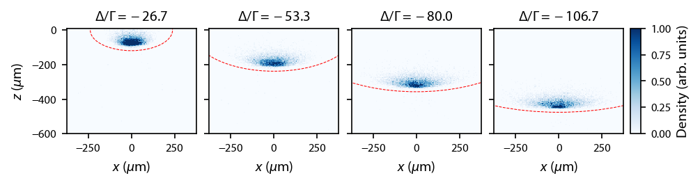
Now plot it up, with the ellipse indicating when the Zeeman shift from the magnetic field gradient equals the detuning

from matplotlib.patches import Ellipse

fig, ax = plt.subplots(1, 4, figsize=(6.5, 1.625))

clims = [43, 35, 30, 25]
for ii in range(4):
    # Want to adjust scale for the increasing size of the MOT.  I thought this was clever:
    counts, bins = np.histogram(imgs[ii].flatten(), bins=np.arange(10, 50, 1))

    im = ax[ii].imshow(imgs[ii].T/(2.5*bins[np.argmax(counts)]), origin='bottom',
                       extent=(np.amin(x_edges), np.amax(x_edges),
                               np.amin(z_edges), np.amax(z_edges)),
                       cmap='Blues', clim=(0, 1))
    ax[ii].set_title('$\Delta/\Gamma = %.1f$'%dets[ii])
    ax[ii].set_xlabel('$x$ ($\mu$m)')

    ellip = Ellipse(xy=(0,0),
                    width=4*dets[ii]/alpha*(1e4*x0),
                    height=2*dets[ii]/alpha*(1e4*x0),
                    linestyle='--',
                    linewidth=0.5,
                    facecolor='none',
                    edgecolor='red')

    ax[ii].add_patch(ellip)
    if ii>0:
        ax[ii].yaxis.set_ticklabels('')

fig.subplots_adjust(left=0.08, bottom=0.12, top=0.97, right=0.9)

pos = ax[-1].get_position()
cbar_ax = fig.add_axes([0.91, pos.y0, 0.015, pos.y1-pos.y0])
fig.colorbar(im, cax=cbar_ax)
cbar_ax.set_ylabel('Density (arb. units)')

ax[0].set_ylabel('$z$ ($\mu$m)')

Text(0, 0.5, '$z$ ($\\mu$m)')