Adiabatic Rapid Passage

This example covers an example with both laser frequency and amplitude modulation: rapid adiabatic passage. It reproduces Fig. 2 from T. Lu, X. Miao, and H. Metcalf, “Bloch theorem on the Bloch sphere” Physical Review A 71, 061405(R) (2005), http://dx.doi.org/10.1103/PhysRevA.71.061405

import numpy as np
import matplotlib.pyplot as plt
from scipy.integrate import solve_ivp
import pylcp
from pylcp.common import progressBar

Code the basic Hamiltonian

The Hamiltonian is a simple two-state Hamiltonian. Here, we code up a method to return the time-dependent Hamiltonian matrix to evolve it with the Schrodinger equation. We take the modulation to be the same as in Lu, et. al., above: \(\Omega(t) = \Omega_0\sin(\omega_m t)\) and \(\Delta=\Delta_0\cos(\omega_m t)\).

def H(t, Delta0, Omega0, omegam):
    Delta = Delta0*np.cos(omegam*t)
    Omega = Omega0*np.sin(omegam*t)

    return 1/2*np.array([[Delta, Omega], [Omega, -Delta]])

Define the problem in pylcp

Unlike the above Hamiltonian, which is clearly time dependent, the only time dependence available to us in pylcp is through the fields. First, we need to remember for the amplitude modulation that \(I/I_{\rm sat} = 2\Omega^2/\Gamma^ = 2[\Omega_0\sin(\omega_m t)]^2/\Gamma^2\). Second, we need to frequency modulate the laser beams. Remember that if the lasers have a temporal phase \(\phi\), the frequency is \(\omega = \frac{d\phi}{dt}\). Thus, if the detuning \(\Delta(t)\) is specified, then \(\phi = \int \Delta (t)\ dt\). pylcp contains a built-in integrator in order to convert the detuning to a phase, but it might not always be reliable. So you can also reproduce the detuning by modulating the phase \(\phi\). To reproduce the \(\Delta(t) = \Delta_0\cos(\omega_m t)\), we need \(\phi = \Delta_0/\omega_m\sin(\omega_m t)\).

def return_lasers(Delta0, Omega0, omegam):
    laserBeams = pylcp.laserBeams([
        {'kvec':np.array([1., 0., 0.]),
         'pol':np.array([0., 0., 1.]),
         'pol_coord':'cartesian',
         'delta': lambda t: Delta0*np.cos(omegam*t),
         'phase': 0,#lambda t: Delta0/omegam*np.sin(omegam*t),
         's': lambda R, t: 2*(Omega0*np.sin(omegam*t))**2
        }])

    return laserBeams

magField = lambda R: np.zeros(R.shape)

# Now define the extremely simple Hamiltonian:
Hg = np.array([[0.]])
mugq = np.array([[[0.]], [[0.]], [[0.]]])
He = np.array([[0.]])
mueq = np.array([[[0.]], [[0.]], [[0.]]])
dijq = np.array([[[0.]], [[1.]], [[0.]]])

gamma = 1.

hamiltonian = pylcp.hamiltonian(Hg, He, mugq, mueq, dijq, gamma=gamma)
hamiltonian.print_structure()

[[((<g|H_0|g> 1x1), (<g|mu_q|g> 1x1)) (<g|d_q|e> 1x1)]
 [(<e|d_q|g> 1x1) ((<e|H_0|e> 1x1), (<e|mu_q|e> 1x1))]]

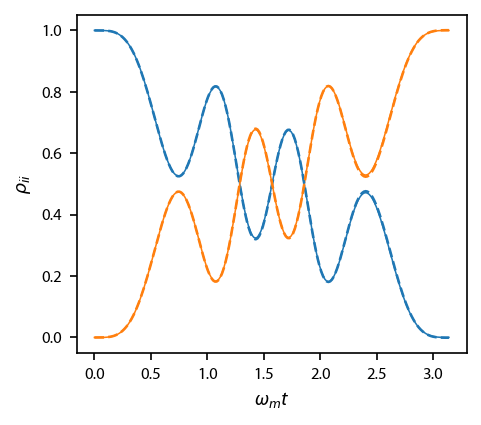
Evolve a single state

We solve with both the Schrodinger Equation and the OBEs. We can play with the modulation parameters (\(\Delta_0\), \(\Omega_0\), \(\omega_m\)), and see how the result chanages.

Delta0 = 5.
Omega0 = 10.
omegam = 1.

t = np.linspace(0., np.pi/omegam, 201)
sol_SE = solve_ivp(lambda t, y: -1j*H(t, Delta0, Omega0, omegam)@y, [0, np.pi/omegam],
                   np.array([1., 0.], dtype='complex128'), t_eval=t)

laserBeams = return_lasers(Delta0, Omega0, omegam)
obe = pylcp.obe(laserBeams, magField, hamiltonian)
obe.ev_mat['decay'] = np.zeros(obe.ev_mat['decay'].shape) # Turn off damping to compare to Schrodinger Equation.
obe.set_initial_rho_from_populations(np.array([1., 0.]))
sol_OBE = obe.evolve_density([0, np.pi/omegam], t_eval=t)

Plot it up. Dashed is OBEs from pylcp and solid is the Schrodiner equation. Orange is the \(|1\rangle\) state; blue is the \(|0\rangle\) state.

fig, ax = plt.subplots(1, 1)
ax.plot(sol_SE.t, np.abs(sol_SE.y[0])**2, linewidth=0.75)
ax.plot(sol_SE.t, np.abs(sol_SE.y[1])**2, linewidth=0.75)
ax.plot(sol_OBE.t, np.real(sol_OBE.rho[0, 0]), '--', color='C0', linewidth=1.25)
ax.plot(sol_OBE.t, np.real(sol_OBE.rho[1, 1]), '--', color='C1', linewidth=1.25)
ax.set_xlabel('$\omega_m t$')
ax.set_ylabel('$\\rho_{ii}$');

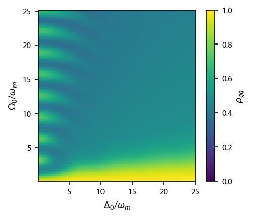
Reproduce Fig. 2

This involves scanning over \(\Delta_0\) and \(\Omega_0\). This takes a long time, only because there is a fair amount of overhead in regenerating the optical Bloch equations on every iteration.

Delta0s = np.arange(0.25, 25.1, 0.25)
Omega0s = np.arange(0.25, 25.1, 0.25)
t = np.linspace(0., np.pi, 201)

DELTA0S, OMEGA0S = np.meshgrid(Delta0s, Omega0s)

it = np.nditer([DELTA0S, OMEGA0S, None])

progress = progressBar()

for (Delta0, Omega0, rhogg) in it:
    del laserBeams

    # Set up new laser beams:
    laserBeams = return_lasers(Delta0, Omega0, omegam)

    # Set up OBE:
    obe = pylcp.obe(laserBeams, magField, hamiltonian)
    obe.ev_mat['decay'] = np.zeros(obe.ev_mat['decay'].shape) # Turn off damping to compare to Schrodinger Equation.
    obe.set_initial_rho_from_populations(np.array([1., 0.]))

    # Solve:
    sol_OBE = obe.evolve_density([0, np.pi], t_eval=t)

    # Save result:
    rhogg[...] = np.real(sol_OBE.rho[0, 0, -1])

    # Update progress bar:
    progress.update((it.iterindex+1)/it.itersize)

RHOGG = it.operands[2]

Completed in 8:02.

Plot it up:

dDelta0 = np.mean(np.diff(Delta0s))
dOmega0 = np.mean(np.diff(Omega0s))
fig, ax = plt.subplots(1, 1)
im = ax.imshow(RHOGG, origin='lower',
               extent=(np.amin(Delta0s)-dDelta0/2, np.amax(Delta0s)+dDelta0/2,
                       np.amin(Omega0s)-dOmega0/2, np.amax(Omega0s)+dOmega0/2),
               aspect='auto')
ax_cbar = plt.colorbar(im)
ax_cbar.set_label('$\\rho_{gg}$')
ax.set_xlabel('$\Delta_0/\omega_m$')
ax.set_ylabel('$\Omega_0/\omega_m$');

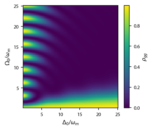
Add in damping

These two cells are exactly the same as above, except the user must now specify \(\omega_m/\Gamma\) (\(\Gamma=1\)) and we merely comment out the line that eliminate the damping part of the OBEs.

omegam = 2
Delta0s = np.arange(0.25, 25.1, 0.25) # These will be normalized to the value of omegam
Omega0s = np.arange(0.25, 25.1, 0.25)
t = np.linspace(0., np.pi/omegam, 201)

DELTA0S, OMEGA0S = np.meshgrid(Delta0s, Omega0s)

it = np.nditer([DELTA0S, OMEGA0S, None])

progress = progressBar()

for (Delta0, Omega0, rhogg) in it:
    # Set up new laser beams:
    laserBeams = return_lasers(omegam*Delta0, omegam*Omega0, omegam)

    # Set up OBE:
    obe = pylcp.obe(laserBeams, magField, hamiltonian)
    obe.set_initial_rho_from_populations(np.array([1., 0.]))

    # Solve:
    sol_OBE = obe.evolve_density([0, np.pi/omegam], t_eval=t)

    # Save result:
    rhogg[...] = np.real(sol_OBE.rho[0, 0, -1])

    # Update progress bar:
    progress.update((it.iterindex+1)/it.itersize)

RHOGG = it.operands[2]

Completed in 7:22.

Plot it up:

dDelta0 = np.mean(np.diff(Delta0s))
dOmega0 = np.mean(np.diff(Omega0s))
fig, ax = plt.subplots(1, 1)
im = ax.imshow(RHOGG, origin='lower',
               extent=(np.amin(Delta0s)-dDelta0/2, np.amax(Delta0s)+dDelta0/2,
                       np.amin(Omega0s)-dOmega0/2, np.amax(Omega0s)+dOmega0/2),
               aspect='auto', clim=(0, 1))
ax_cbar = plt.colorbar(im)
ax_cbar.set_label('$\\rho_{gg}$')
ax.set_xlabel('$\Delta_0/\omega_m$')
ax.set_ylabel('$\Omega_0/\omega_m$');