\(F=0\rightarrow F'=1\) 1D molasses
This example covers calculating the forces in a one-dimensional optical molasses using the optical bloch equations. This example does the boring thing and checks that everything is working on the \(F=0\rightarrow F=1\) transition, which of course has no sub-Doppler effect. It is a bit more complicated than the two level molasses example, as now different kinds of polarizations and \(\hat{k}\) vectors can be used. By exploring multiple combinations, we can verify that the OBEs are working properly.
It first checks the force along the \(\hat{z}\)-direction. One should look to see that things agree with what one expects whether or not one puts the detuning on the lasers or on the Hamilonian. One should also look at whether the force depends on transforming the OBEs into the real/imaginary components.
[1]:
import numpy as np
import matplotlib.pyplot as plt
import pylcp
Define the problem
We start with defining multiple laser beam polarizations. We store these in a dictionary, keyed by the polarization. In this example, we can also specify the rotating frame, and how the lasers might have a residual oscillation in that frame. The total detuning is the sum of the detuning of the lasers and hamiltonian (see the associated paper). Answers should of course be independent, but computational speed may not be.
[2]:
laser_det = 0.
ham_det = -2.
s = 1.25

laserBeams = {}
laserBeams['$\\sigma^+\\sigma^+$'] = pylcp.laserBeams([
    {'kvec':np.array([0., 0., 1.]), 'pol':np.array([0., 0., 1.]),
     'pol_coord':'spherical', 'delta':laser_det, 's':s},
    {'kvec':np.array([0., 0., -1.]), 'pol':np.array([0., 0., 1.]),
     'pol_coord':'spherical', 'delta':laser_det, 's':s},
    ], beam_type=pylcp.infinitePlaneWaveBeam)

laserBeams['$\\sigma^+\\sigma^-$'] = pylcp.laserBeams([
    {'kvec':np.array([0., 0., 1.]), 'pol':np.array([0., 0., 1.]),
     'pol_coord':'spherical', 'delta':laser_det, 's':s},
    {'kvec':np.array([0., 0., -1.]), 'pol':np.array([1., 0., 0.]),
     'pol_coord':'spherical', 'delta':laser_det, 's':s},
    ], beam_type=pylcp.infinitePlaneWaveBeam)

laserBeams['$\\pi_x\\pi_x$'] = pylcp.laserBeams([
    {'kvec':np.array([0., 0., 1.]), 'pol':np.array([1., 0., 0.]),
     'pol_coord':'cartesian', 'delta':laser_det, 's':s},
    {'kvec':np.array([0., 0., -1.]), 'pol':np.array([1., 0., 0.]),
     'pol_coord':'cartesian', 'delta':laser_det, 's':s},
    ], beam_type=pylcp.infinitePlaneWaveBeam)

laserBeams['$\\pi_x\\pi_y$'] = pylcp.laserBeams([
    {'kvec':np.array([0., 0., 1.]), 'pol':np.array([1., 0., 0.]),
     'pol_coord':'cartesian', 'delta':laser_det, 's':s},
    {'kvec':np.array([0., 0., -1.]), 'pol':np.array([0., 1., 0.]),
     'pol_coord':'cartesian', 'delta':laser_det, 's':s},
    ], beam_type=pylcp.infinitePlaneWaveBeam)

laserBeams['$\\sigma^+\\sigma^-$'].total_electric_field_gradient(np.array([0., 0., 0.]), 0.)
magField = lambda R: np.zeros(R.shape)

# Hamiltonian for F=0->F=1
Hg, Bgq = pylcp.hamiltonians.singleF(F=0, gF=0, muB=1)
He, Beq = pylcp.hamiltonians.singleF(F=1, gF=1, muB=1)
dijq = pylcp.hamiltonians.dqij_two_bare_hyperfine(0, 1)
ham_F0_to_F1 = pylcp.hamiltonian(Hg, He - ham_det*np.eye(3), Bgq, Beq, dijq)
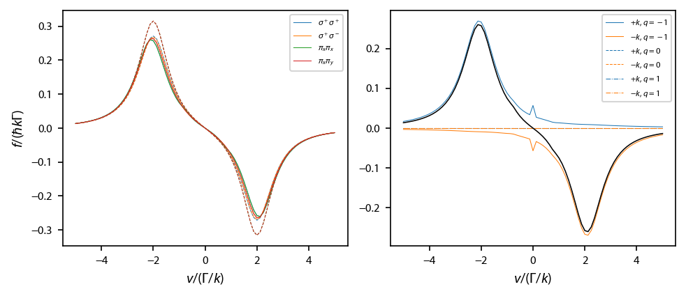
Calculate the equilibrium force profile
This checks to see that the rate equations and OBE agree for \(F=0\rightarrow F'=1\), two-state solution:
[3]:
obe={}
rateeq={}

# Define a v axis:
v = np.arange(-5.0, 5.1, 0.125)

for jj, key in enumerate(laserBeams.keys()):
    print('Working on %s:' % key)
    rateeq[key] = pylcp.rateeq(laserBeams[key], magField, ham_F0_to_F1)
    obe[key] = pylcp.obe(laserBeams[key], magField, ham_F0_to_F1,
                         transform_into_re_im=False, include_mag_forces=False)

    # Generate a rateeq model of what's going on:
    rateeq[key].generate_force_profile(
        [np.zeros(v.shape), np.zeros(v.shape), np.zeros(v.shape)],
        [np.zeros(v.shape), np.zeros(v.shape), v],
        name='molasses'
    )

    obe[key].generate_force_profile(
        [np.zeros(v.shape), np.zeros(v.shape), np.zeros(v.shape)],
        [np.zeros(v.shape), np.zeros(v.shape), v],
        name='molasses', deltat_tmax=2*np.pi*100, deltat_v=4, itermax=1000,
        progress_bar=True,
    )
Working on $\sigma^+\sigma^+$:
Completed in 42.48 s.
Working on $\sigma^+\sigma^-$:
Completed in 50.15 s.
Working on $\pi_x\pi_x$:
Completed in 49.28 s.
Working on $\pi_x\pi_y$:
Completed in 45.20 s.
Plot up the results:
[4]:
fig, ax = plt.subplots(1, 2, num='Optical Molasses F=0->F1', figsize=(6.5, 2.75))
for jj, key in enumerate(laserBeams.keys()):
    ax[0].plot(obe[key].profile['molasses'].V[2],
               obe[key].profile['molasses'].F[2],
               label=key, linewidth=0.5, color='C%d'%jj)
    ax[0].plot(rateeq[key].profile['molasses'].V[2],
               rateeq[key].profile['molasses'].F[2], '--',
               linewidth=0.5, color='C%d'%jj)
ax[0].legend(fontsize=6)
ax[0].set_xlabel('$v/(\Gamma/k)$')
ax[0].set_ylabel('$f/(\hbar k \Gamma)$')

key = '$\\sigma^+\\sigma^+$'
types = ['-', '--', '-.']
for q in range(3):
    ax[1].plot(v, obe[key].profile['molasses'].fq['g->e'][2, :, q, 0], types[q],
            linewidth=0.5, color='C0', label='$+k$, $q=%d$'%(q-1))
    ax[1].plot(v, obe[key].profile['molasses'].fq['g->e'][2, :, q, 1], types[q],
            linewidth=0.5, color='C1', label='$-k$, $q=%d$'%(q-1))
ax[1].plot(v, obe[key].profile['molasses'].F[2], 'k-',
           linewidth=0.75)
ax[1].legend(fontsize=6)
ax[1].set_xlabel('$v/(\Gamma/k)$')
fig.subplots_adjust(left=0.08, wspace=0.15)
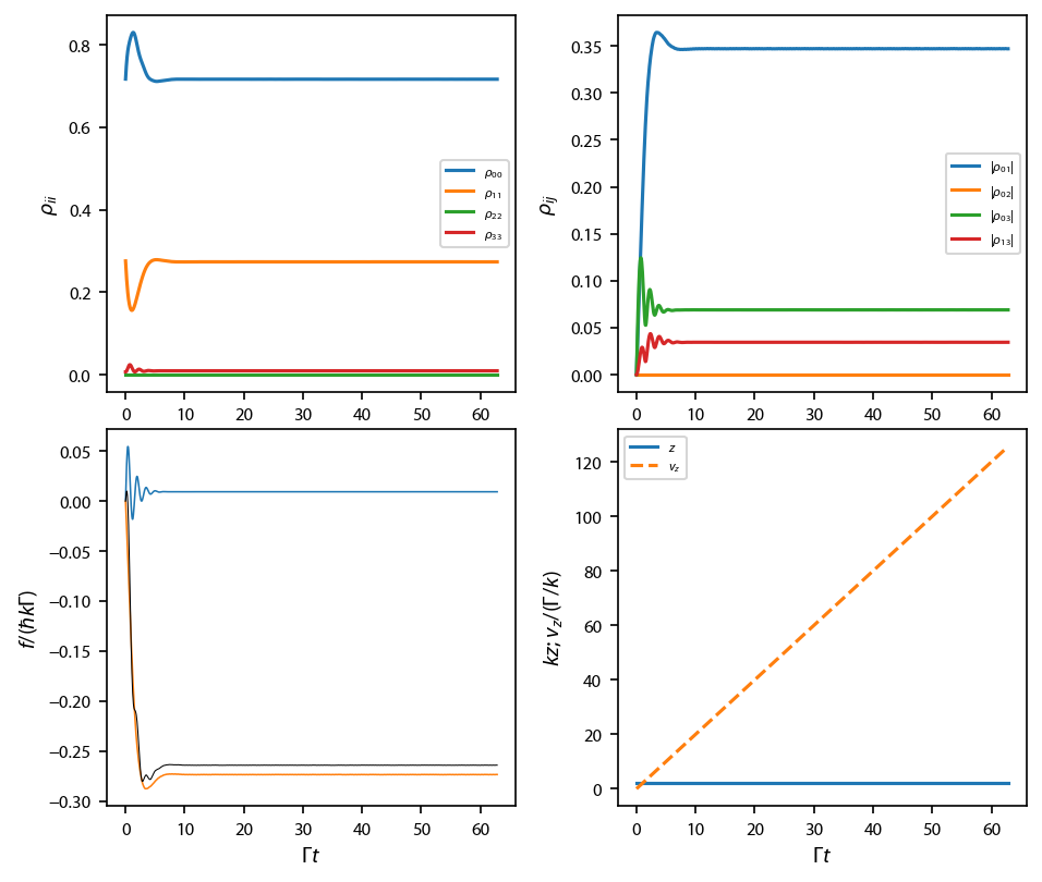
Run a simulation at resonance
This allows us to see what the coherences and such are doing.
[5]:
v_i=-(ham_det+laser_det)
key = '$\\sigma^+\\sigma^-$'

obe[key] = pylcp.obe(laserBeams[key], magField, ham_F0_to_F1,
                     transform_into_re_im=True)

obe[key].set_initial_position_and_velocity(
    np.array([0., 0., 0.]), np.array([0., 0., v_i])
    )
rho0 = np.zeros((obe[key].hamiltonian.n**2,), dtype='complex128')
rho0[0] = 1.

if v_i==0 or np.abs(2*np.pi*20/v_i)>500:
    t_max = 500
else:
    t_max = 2*np.pi*20/np.abs(v_i)

obe[key].set_initial_rho_from_rateeq()
obe[key].evolve_density(t_span=[0, t_max], t_eval=np.linspace(0, t_max, 1001),)

f, flaser, flaser_q, f_mag = obe[key].force(obe[key].sol.r, obe[key].sol.t,
                                            obe[key].sol.rho, return_details=True)

fig, ax = plt.subplots(2, 2, num='OBE F=0->F1', figsize=(6.25, 5.5))
ax[0, 0].plot(obe[key].sol.t, np.real(obe[key].sol.rho[0, 0]), label='$\\rho_{00}$')
ax[0, 0].plot(obe[key].sol.t, np.real(obe[key].sol.rho[1, 1]), label='$\\rho_{11}$')
ax[0, 0].plot(obe[key].sol.t, np.real(obe[key].sol.rho[2, 2]), label='$\\rho_{22}$')
ax[0, 0].plot(obe[key].sol.t, np.real(obe[key].sol.rho[3, 3]), label='$\\rho_{33}$')
ax[0, 0].legend(fontsize=6)

ax[0, 1].plot(obe[key].sol.t, np.abs(obe[key].sol.rho[0, 1]), label='$|\\rho_{01}|$')
ax[0, 1].plot(obe[key].sol.t, np.abs(obe[key].sol.rho[0, 2]), label='$|\\rho_{02}|$')
ax[0, 1].plot(obe[key].sol.t, np.abs(obe[key].sol.rho[0, 3]), label='$|\\rho_{03}|$')
ax[0, 1].plot(obe[key].sol.t, np.abs(obe[key].sol.rho[1, 3]), label='$|\\rho_{13}|$')
ax[0, 1].legend(fontsize=6)

ax[1, 0].plot(obe[key].sol.t, flaser['g->e'][2, 0], '-', linewidth=0.75)
ax[1, 0].plot(obe[key].sol.t, flaser['g->e'][2, 1], '-', linewidth=0.75)
ax[1, 0].plot(obe[key].sol.t, f[2], 'k-', linewidth=0.5)

ax[1, 1].plot(obe[key].sol.t, obe[key].sol.v[-1], '-', label='$z$')
ax[1, 1].plot(obe[key].sol.t, obe[key].sol.r[-1], '--', label='$v_z$')
ax[1, 1].legend(fontsize=6);

ax[0, 0].set_ylabel('$\\rho_{ii}$')
ax[0, 1].set_ylabel('$\\rho_{ij}$')
ax[1, 0].set_ylabel('$f/(\hbar k \Gamma)$')
ax[1, 1].set_ylabel('$kz$; $v_z/(\Gamma/k)$')

ax[1, 0].set_xlabel('$\Gamma t$')
ax[1, 1].set_xlabel('$\Gamma t$')

fig.subplots_adjust(left=0.08, bottom=0.1, wspace=0.25)
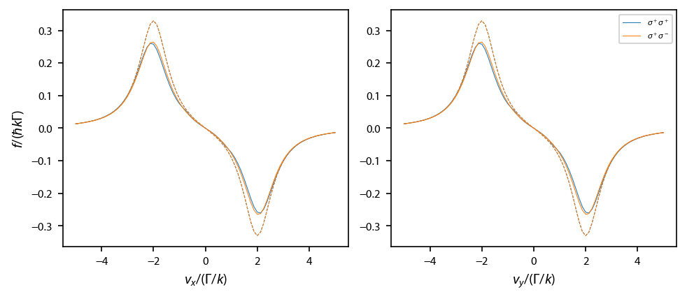
Finally, calculate \(\mathbf{f}\) when \(\mathbf{k}\) is along \(\mathbf{x}\) and \(\mathbf{y}\)
This helps to make sure that everything is coded properly.
[6]:
laserBeams = {}
laserBeams['x'] = {}
laserBeams['x']['$\\sigma^+\\sigma^+$'] = pylcp.laserBeams([
    {'kvec':np.array([ 1., 0., 0.]), 'pol':+1, 'delta':laser_det, 's':s},
    {'kvec':np.array([-1., 0., 0.]), 'pol':-1, 'delta':laser_det, 's':s},
    ])
laserBeams['x']['$\\sigma^+\\sigma^-$'] = pylcp.laserBeams([
    {'kvec':np.array([ 1., 0., 0.]), 'pol':+1, 'delta':laser_det, 's':s},
    {'kvec':np.array([-1., 0., 0.]), 'pol':+1, 'delta':laser_det, 's':s},
    ])
laserBeams['y'] = {}
laserBeams['y']['$\\sigma^+\\sigma^+$'] = pylcp.laserBeams([
    {'kvec':np.array([0.,  1., 0.]), 'pol':+1, 'delta':laser_det, 's':s},
    {'kvec':np.array([0., -1., 0.]), 'pol':-1, 'delta':laser_det, 's':s},
    ])
laserBeams['y']['$\\sigma^+\\sigma^-$'] = pylcp.laserBeams([
    {'kvec':np.array([0.,  1., 0.]), 'pol':+1, 'delta':laser_det, 's':s},
    {'kvec':np.array([0., -1., 0.]), 'pol':+1, 'delta':laser_det, 's':s},
    ])

obe = {}
rateeq = {}
for coord_key in laserBeams:
    obe[coord_key] = {}
    rateeq[coord_key] = {}
    for pol_key in laserBeams[coord_key]:
        print('Working on %s along %s.' % (pol_key, coord_key))
        rateeq[coord_key][pol_key] = pylcp.rateeq(laserBeams[coord_key][pol_key],
                                                  magField, ham_F0_to_F1)
        obe[coord_key][pol_key] = pylcp.obe(laserBeams[coord_key][pol_key],
                                            magField, ham_F0_to_F1,
                                            transform_into_re_im=False,
                                            include_mag_forces=True)

        if coord_key is 'x':
            V = [v, np.zeros(v.shape), np.zeros(v.shape)]
        elif coord_key is 'y':
            V = [np.zeros(v.shape), v, np.zeros(v.shape)]
        R = np.zeros((3,)+v.shape)
        # Generate a rateeq model of what's going on:
        rateeq[coord_key][pol_key].generate_force_profile(
            R, V, name='molasses'
        )

        obe[coord_key][pol_key].generate_force_profile(
            R, V, name='molasses', deltat_tmax=2*np.pi*100, deltat_v=4,
            itermax=1000, progress_bar=True
        )
Working on $\sigma^+\sigma^+$ along x.
Completed in 49.64 s.
Working on $\sigma^+\sigma^-$ along x.
Completed in 52.31 s.
Working on $\sigma^+\sigma^+$ along y.
Completed in 57.35 s.
Working on $\sigma^+\sigma^-$ along y.
Completed in 52.62 s.
Plot up these results:
[7]:
fig, ax = plt.subplots(1, 2, num='Optical Molasses F=0->F1', figsize=(6.5, 2.75))
for ii, coord_key in enumerate(laserBeams.keys()):
    for jj, pol_key in enumerate(laserBeams[coord_key].keys()):
        ax[ii].plot(obe[coord_key][pol_key].profile['molasses'].V[ii],
                   obe[coord_key][pol_key].profile['molasses'].F[ii],
                   label=pol_key, linewidth=0.5, color='C%d'%jj)
        ax[ii].plot(rateeq[coord_key][pol_key].profile['molasses'].V[ii],
                    rateeq[coord_key][pol_key].profile['molasses'].F[ii], '--',
                    linewidth=0.5, color='C%d'%jj)
ax[1].legend(fontsize=6)
ax[0].set_xlabel('$v_x/(\Gamma/k)$')
ax[1].set_xlabel('$v_y/(\Gamma/k)$')
ax[0].set_ylabel('$f/(\hbar k \Gamma)$')
fig.subplots_adjust(left=0.08, wspace=0.15)