\(F=2 \rightarrow F'=3\) 1D molasses

This example covers calculating the forces in a one-dimensional optical molasses using the optical bloch equations. It attempts to reproduce several figures from Ungar, P. J., Weiss, D. S., Riis, E., & Chu, S. “Optical molasses and multilevel atoms: theory.” Journal of the Optical Society of America B, 6 2058 (1989). http://doi.org/10.1364/JOSAB.6.002058

import numpy as np
import matplotlib.pyplot as plt
from mpl_toolkits.axes_grid1.inset_locator import inset_axes
import pylcp
import scipy.constants as cts
from pylcp.common import progressBar
import lmfit

Define the problem

Unager, et. al. focus on sodium, so we first find the mass parameter for \(^{23}\)Na:

atom = pylcp.atom('23Na')
mass = (atom.state[2].gamma*atom.mass)/(cts.hbar*(100*2*np.pi*atom.transition[1].k)**2)
print(mass)

195.87538720801354

As with all other examples, we need to define the Hamiltonian, lasers, and magnetic field. Here, we will write methods to return the Hamiltonian and the lasers in order to sweep their parameters. Note that the magnetic field is always zero, so we define it as such. Lastly, we make a dictionary of different polarizations that we will explore in this example.

def return_hamiltonian(Fl, Delta):
    Hg, Bgq = pylcp.hamiltonians.singleF(F=Fl, gF=0, muB=1)
    He, Beq = pylcp.hamiltonians.singleF(F=Fl+1, gF=1/(Fl+1), muB=1)
    dijq = pylcp.hamiltonians.dqij_two_bare_hyperfine(Fl, (Fl+1))
    hamiltonian = pylcp.hamiltonian(Hg, -Delta*np.eye(He.shape[0])+He, Bgq, Beq, dijq, mass=mass)

    return hamiltonian

# Now, make 1D laser beams:
def return_lasers(delta, s, pol):
    if pol[0][2]>0 or pol[0][1]>0:
        pol_coord = 'spherical'
    else:
        pol_coord = 'cartesian'

    return pylcp.laserBeams([
        {'kvec':np.array([0., 0., 1.]), 'pol':pol[0],
         'pol_coord':pol_coord, 'delta':delta, 's':s},
        {'kvec':np.array([0., 0., -1.]), 'pol':pol[1],
         'pol_coord':pol_coord, 'delta':delta, 's':s},
        ], beam_type=pylcp.infinitePlaneWaveBeam)

magField = pylcp.constantMagneticField(np.array([0., 0., 0.]))

# Now make a bunch of polarization keys:
pols = {'$\\sigma^+\\sigma^-$':[np.array([0., 0., 1.]), np.array([1., 0., 0.])],
        '$\\sigma^+\\sigma^+$':[np.array([0., 0., 1.]), np.array([0., 0., 1.])]}

phi = [0, np.pi/4, np.pi/2]
phi_keys = ['$\phi=0$', '$\phi=\pi/4$', '$\phi=\pi/2$']
for phi_i, key_beam in zip(phi, phi_keys):
        pols[key_beam] = [np.array([1., 0., 0.]), np.array([np.cos(phi_i), np.sin(phi_i), 0.])]

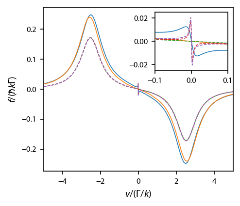
Make a basic force profile

This is not contained in Ungar, et. al., but it makes a nice figure that contains most of the essential elements thereof. We start by creating, using our functions defined above, a set of lasers, the Hamiltonian, and then the set of optical Bloch equations for each polarization specified in the dictionary defined above.

det = -2.5
s = 1.0

hamiltonian = return_hamiltonian(2, det)

v = np.concatenate((np.arange(0.001, 0.01, 0.001),
                    np.arange(0.01, 0.02, 0.002),
                    np.arange(0.02, 0.03, 0.005),
                    np.arange(0.03, 0.1, 0.01),
                    np.arange(0.1, 5.1, 0.1)))

obe = {}
for key_beam in pols:
    laserBeams = return_lasers(0., s, pol=pols[key_beam])

    obe[key_beam] = pylcp.obe(
        laserBeams, magField, hamiltonian,
        include_mag_forces=False, transform_into_re_im=True
    )

    obe[key_beam].generate_force_profile(
        [np.zeros(v.shape), np.zeros(v.shape), np.zeros(v.shape)],
        [np.zeros(v.shape), np.zeros(v.shape), v],
        name='molasses', deltat_v=4, deltat_tmax=2*np.pi*5000, itermax=1000,
        rel=1e-8, abs=1e-10, progress_bar=True
    )

Completed in 7:11.
Completed in 3:25.
Completed in 7:19.
Completed in 7:49.
Completed in 7:43.

Plot it up:

fig, ax = plt.subplots(1, 1)
axins = inset_axes(ax, width=1.0, height=0.8)
for key in obe:
    if 'phi' in key:
        linestyle='--'
    else:
        linestyle='-'

    ax.plot(np.concatenate((-v[::-1], v)),
            np.concatenate((-obe[key].profile['molasses'].F[2][::-1],
                            obe[key].profile['molasses'].F[2])),
            label=pols[key], linestyle=linestyle,
            linewidth=0.75
            )
    axins.plot(np.concatenate((-v[::-1], v)),
               np.concatenate((-obe[key].profile['molasses'].F[2][::-1],
                               obe[key].profile['molasses'].F[2])),
            label=pols[key], linestyle=linestyle,
            linewidth=0.75
            )

ax.set_xlim(-5, 5)
ax.set_xlabel('$v/(\Gamma/k)$')
ax.set_ylabel('$f/(\hbar k \Gamma)$')
axins.set_xlim(-0.1, 0.1)
axins.set_ylim(-0.025, 0.025);

Reproduce various figures

Figure 6

This figure compares the force for various polarizations. To make it, we first make each OBE individually, and save the resulting forces. Note that in Ungar, et. al., they define their velocity scale through \(m v_0^2 = \hbar\Gamma\), resulting in forces in terms of \(M v_0 \Gamma\). Compared to us, they measure their velocities in terms of

\[\frac{v_0}{k/\Gamma} = \sqrt{\frac{\hbar\Gamma}{m}}\frac{k}{\Gamma} = \sqrt{\frac{\hbar k^2}{\Gamma m}} = \sqrt{\bar{m}}\]

Likewise, the force ratio,

\[\frac{M v_0 \Gamma}{\hbar k \Gamma} = \frac{M\sqrt{\hbar\Gamma}}{\hbar k} = \sqrt{\frac{M\Gamma}{\hbar k^2}} = \sqrt{\bar{m}}\]

det = -2.73
s = 1.25

v = np.concatenate((np.array([0.0]), np.logspace(-2, np.log10(4), 20)))/np.sqrt(mass)

keys_of_interest = ['$\\sigma^+\\sigma^+$', '$\\sigma^+\\sigma^-$',
                    '$\phi=0$', '$\phi=\pi/2$']

F = {}
for key in keys_of_interest:
    laserBeams = return_lasers(0., s, pol=pols[key])
    hamiltonian = return_hamiltonian(2, det)

    obe = pylcp.obe(laserBeams, magField, hamiltonian,
                    transform_into_re_im=True)

    obe.generate_force_profile(
        [np.zeros(v.shape), np.zeros(v.shape), np.zeros(v.shape)],
        [np.zeros(v.shape), np.zeros(v.shape), v],
        name='molasses', deltat_tmax=2*np.pi*1000, deltat_v=4, itermax=10,
        progress_bar=True
    )

    F[key] = obe.profile['molasses'].F[2]

Completed in 6:46.
Completed in 3:59.
Completed in 7:42.
Completed in 8:05.

Plot it up.

fig, ax = plt.subplots(1, 1, num="Forces; F=2 to F=3")
for key in keys_of_interest:
    ax.plot(v*np.sqrt(mass), -1e3*F[key]/np.sqrt(mass), label=key)
ax.set_xlabel('$v/\sqrt{\hbar\Gamma/m}$')
ax.set_ylabel('$f/\sqrt{\hbar m \Gamma^3}$')
ax.legend(fontsize=8)
ax.set_xlim((0, 4.))
ax.set_ylim((0, 2.));

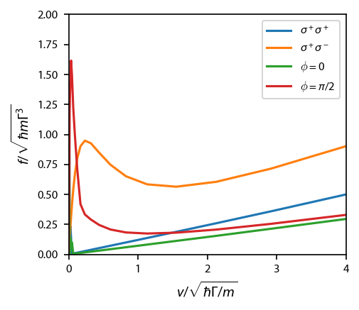
Figure 7

Compare the two-level vs. the corkscrew at large velocities.

v = np.concatenate((np.arange(0, 1.5, 0.2),
                    np.arange(0.2, 50., 1.5)))/np.sqrt(mass)

s = 1.25
det = -2.73

keys_of_interest = ['$\\sigma^+\\sigma^+$', '$\\sigma^+\\sigma^-$']

f = {}
for key in keys_of_interest:
    laserBeams = return_lasers(0., s, pol=pols[key])
    hamiltonian = return_hamiltonian(2, det)

    obe = pylcp.obe(laserBeams, magField, hamiltonian,
                    transform_into_re_im=True)

    obe.generate_force_profile(
        [np.zeros(v.shape), np.zeros(v.shape), np.zeros(v.shape)],
        [np.zeros(v.shape), np.zeros(v.shape), v],
        name='molasses', deltat_tmax=2*np.pi*100, deltat_v=4, itermax=1000,
        progress_bar=True
    )

    f[key] = obe.profile['molasses'].F[2]

Completed in 5:15.
Completed in 1:24.

Plot it up

fig, ax = plt.subplots(1, 1)
for key in keys_of_interest:
    ax.plot(v*np.sqrt(mass), -1e3*f[key]/np.sqrt(mass), label=key)
ax.set_xlabel('$v/\sqrt{\hbar\Gamma/m}$')
ax.set_ylabel('$F/\sqrt{\hbar m \Gamma^3}$')
ax.set_ylim((0, 25))
ax.set_xlim((0, 50))
ax.legend(fontsize=8);

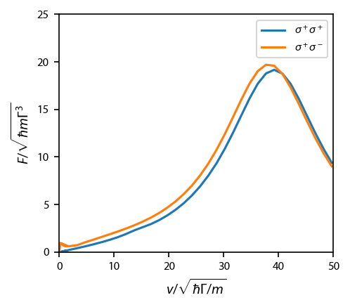
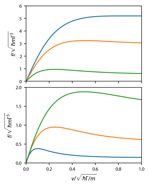
Figure 8

We run the detuning and saturation parameter for the corkscrew model.

dets = [-1.0, -1.37, -2.73]
intensities = [0.5, 1.25, 2.5]
key = '$\\sigma^+\\sigma^-$'

v = np.arange(0.0, 1.025, 0.025)/np.sqrt(mass)
F_dets = [None]*3
for ii, det in enumerate(dets):
    laserBeams = return_lasers(0., intensities[1], pol=pols[key])
    hamiltonian = return_hamiltonian(2, det)

    obe = pylcp.obe(laserBeams, magField, hamiltonian)

    obe.generate_force_profile(
        [np.zeros(v.shape), np.zeros(v.shape), np.zeros(v.shape)],
        [np.zeros(v.shape), np.zeros(v.shape), v],
        name='molasses', deltat_tmax=2*np.pi*100, deltat_v=4, itermax=1000,
        progress_bar=True
    )

    F_dets[ii] = obe.profile['molasses'].F[2]

F_intensities = [None]*3
for ii, s in enumerate(intensities):
    laserBeams = return_lasers(0., s, pol=pols[key])
    hamiltonian = return_hamiltonian(2, dets[-1])

    obe = pylcp.obe(laserBeams, magField, hamiltonian)

    obe.generate_force_profile(
        [np.zeros(v.shape), np.zeros(v.shape), np.zeros(v.shape)],
        [np.zeros(v.shape), np.zeros(v.shape), v],
        name='molasses', deltat_tmax=2*np.pi*100, deltat_v=4, itermax=1000,
        progress_bar=True
    )

    F_intensities[ii] = obe.profile['molasses'].F[2]

Completed in 1:03.
Completed in 1:23.
Completed in 4:36.
Completed in 6:47.
Completed in 4:05.
Completed in 2:15.

Plot it up:

fig, ax = plt.subplots(2, 1, figsize=(3.25, 1.5*2.75))
for (F, det) in zip(F_dets, dets):
    ax[0].plot(v*np.sqrt(mass), -1e3*F/np.sqrt(mass), label='$\delta = %f' % det)
for (F, s) in zip(F_intensities, intensities):
    ax[1].plot(v*np.sqrt(mass), -1e3*F/np.sqrt(mass), label='$s = %f' % s)
ax[1].set_xlabel('$v/\sqrt{\hbar\Gamma/m}$')
ax[0].set_ylabel('$f/\sqrt{\hbar m \Gamma^3}$')
ax[0].set_ylim((0, 6))
ax[0].set_xlim((0, 1))
ax[1].set_ylabel('$f/\sqrt{\hbar m \Gamma^3}$')
ax[1].set_ylim((0, 2))
ax[1].set_xlim((0, 1))

ax[0].xaxis.set_ticklabels('')

fig.subplots_adjust(bottom=0.12, hspace=0.08)

Simulate many atoms and find the temperature:

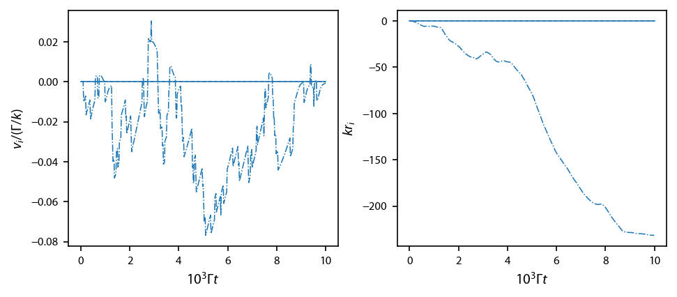
We start with just a single atom just to make sure everything is OK.

tmax = 1e4
det = -2.73
s = 1.25
key =  '$\\sigma^+\\sigma^-$'

laserBeams = return_lasers(0., s, pol=pols[key])
hamiltonian = return_hamiltonian(2, det)

obe = pylcp.obe(laserBeams, magField, hamiltonian,
                include_mag_forces=False)

obe.set_initial_position(np.array([0., 0., 0.]))
obe.set_initial_velocity(np.array([0., 0., 0.]))
obe.set_initial_rho_equally()

obe.evolve_motion(
    [0, tmax],
    t_eval=np.linspace(0, tmax, 501),
    random_recoil=True,
    progress_bar=True,
    max_scatter_probability=0.5,
    record_force=True,
    freeze_axis=[True, True, False]
);

Completed in 30.95 s.

Plot up the test simulation:

fig, ax = plt.subplots(1, 2, figsize=(6.5, 2.75))
ll = 0
styles = ['-', '--', '-.']
for jj in range(3):
    ax[0].plot(obe.sol.t/1e3,
               obe.sol.v[jj], styles[jj],
               color='C%d'%ll, linewidth=0.75)
    ax[1].plot(obe.sol.t/1e3,
               obe.sol.r[jj],
               styles[jj], color='C%d'%ll, linewidth=0.75)

#ax[1].set_ylim(-5., 5.)
ax[0].set_ylabel('$v_i/(\Gamma/k)$')
ax[1].set_ylabel('$k r_i$')
ax[0].set_xlabel('$10^{3} \Gamma t$')
ax[1].set_xlabel('$10^{3} \Gamma t$')
fig.subplots_adjust(left=0.1, wspace=0.22)

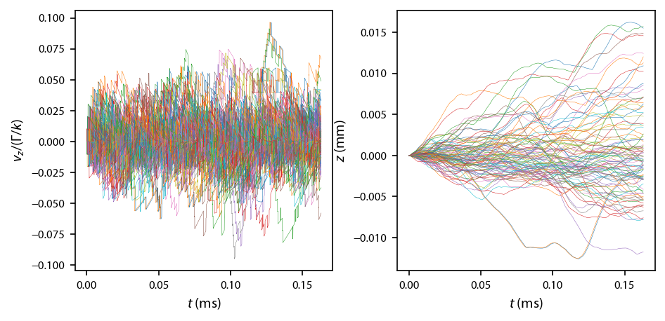
Now run a large sim with 96 atoms:

Non-parallel version:

sols = []
for jj in range(Natoms):
    trap.set_initial_position(np.array([0., 0., 100.]))
    trap.set_initial_velocity(0.0*np.random.randn(3))

    trap.evolve_motion([0, 3e2],
                       t_eval=np.linspace(0, 1e2, 1001),
                       random_recoil=True,
                       recoil_velocity=v_R,
                       progress_bar=True,
                       max_scatter_probability=0.5,
                       record_force=True)

    sols.append(copy.copy(trap.sol))

Parallel version using pathos:

import pathos
if hasattr(obe, 'sol'):
    del obe.sol

t_eval = np.linspace(0, tmax, 5001)

def generate_random_solution(x, tmax=1e4):
    # We need to generate random numbers to prevent solutions from being seeded
    # with the same random number.
    np.random.rand(256*x)
    obe.set_initial_position(np.array([0., 0., 0.]))
    obe.set_initial_velocity(np.array([0., 0., 0.]))
    obe.set_initial_rho_equally()
    obe.evolve_motion(
        [0, tmax],
        t_eval=t_eval,
        random_recoil=True,
        max_scatter_probability=0.5,
        record_force=True,
        freeze_axis=[True, True, False]
    )

    return obe.sol

Natoms = 96
chunksize = 4
sols = []
progress = progressBar()
for jj in range(int(Natoms/chunksize)):
    with pathos.pools.ProcessPool(nodes=4) as pool:
        sols += pool.map(generate_random_solution, range(chunksize))
    progress.update((jj+1)/int(Natoms/chunksize))

Completed in 15:36.

Now, plot all 96 trajectories:

fig, ax = plt.subplots(1, 2, figsize=(6.25, 2.75))

for sol in sols:
    ax[0].plot(sol.t*atom.state[1].tau*1e3,
               sol.v[2], linewidth=0.25)
    ax[1].plot(sol.t*atom.state[1].tau*1e3,
               sol.r[2]/(2*np.pi*0.1*atom.transition[1].k), linewidth=0.25)

for ax_i in ax:
    ax_i.set_xlabel('$t$ (ms)')
ax[0].set_ylabel('$v_z/(\Gamma/k)$')
ax[1].set_ylabel('$z$ (mm)')

fig.subplots_adjust(left=0.1, bottom=0.08, wspace=0.25)

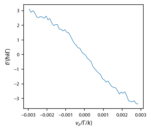
One interesting result from the Unager paper is to look at the average force as a function of position and velocity for the random particles.

allv = np.concatenate([sol.v.T for sol in sols]).T
allF = np.concatenate([sol.F.T for sol in sols]).T

v = np.arange(-.003, 0.003, 0.0001)
vc = v[:-1]+np.mean(np.diff(v))/2

avgFv = np.zeros((3, 3, vc.size))
stdFv = np.zeros((3, 3, vc.size))

for jj in range(3):
    for ii, (v_l, v_r) in enumerate(zip(v[:-1],v[1:])):
        inds = np.bitwise_and(allv[jj] <= v_r, allv[jj] > v_l)
        if np.sum(inds)>0:
            for kk in range(3):
                avgFv[kk, jj, ii] = np.mean(allF[kk, inds])
                stdFv[kk, jj, ii] = np.std(allF[kk, inds])
        else:
            avgFv[:, jj, ii] = np.nan
            avgFv[:, jj, ii] = np.nan

fig, ax = plt.subplots(1, 1)
ax.plot(vc, 1e3*avgFv[2, 2], linewidth=0.75)
ax.set_xlabel('$v_z/\Gamma/k)$')
ax.set_ylabel('$f/(\hbar k \Gamma)$')

Text(0, 0.5, '$f/(\\hbar k \\Gamma)$')

Now, let’s bin the final data and fit it the histogram to extract the temperature.

In this cell, I have included the ability to fit with a two-component Gaussian, but a single component should be sufficient

vs = np.array([sol.v[2] for sol in sols])

xb = np.arange(-0.1, 0.1, 0.005)
fig, ax = plt.subplots(1, 1)
ax.hist(vs[:, 1000::250].flatten(), bins=xb)
x = xb[:-1] + np.diff(xb)/2
y = np.histogram(vs[:, 1000::250].flatten(), bins=xb)[0]

model = lmfit.models.GaussianModel(prefix='A_')# + lmfit.models.GaussianModel(prefix='B_')

params = model.make_params()
params['A_sigma'].value = 0.05
#params['B_sigma'].value = 0.01

ok = y>0
result = model.fit(y[ok], params, x=x[ok], weights=1/np.sqrt(y[ok]))

x_fit = np.linspace(-0.1, 0.1, 101)
ax.plot(x_fit, result.eval(x=x_fit))
ax.set_xlabel('$v/(\Gamma/k)$')
ax.set_ylabel('Counts')

Text(0, 0.5, 'Counts')

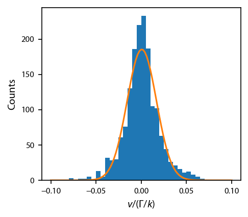
Print the best fit model results:

print('Temperature: %.1f uK'%(2*result.best_values['A_sigma']**2*mass*cts.hbar*atom.state[2].gamma/2/cts.k*1e6))
result

Temperature: 24.2 uK

Model

Model(gaussian, prefix='A_')

Fit Statistics

fitting method	leastsq
# function evals	38
# data points	32
# variables	3
chi-square	123.315114
reduced chi-square	4.25224530
Akaike info crit.	49.1682265
Bayesian info crit.	53.5654342

Variables

name	value	standard error	relative error	initial value	min	max	vary	expression
A_amplitude	7.54346347	0.40047986	(5.31%)	1.0	-inf	inf	True
A_center	6.2493e-04	8.6274e-04	(138.05%)	0.0	-inf	inf	True
A_sigma	0.01622630	7.1807e-04	(4.43%)	0.05	0.00000000	inf	True
A_fwhm	0.03821001	0.00169092	(4.43%)	0.11774100000000001	-inf	inf	False	2.3548200*A_sigma
A_height	185.464796	12.8180580	(6.91%)	7.978846	-inf	inf	False	0.3989423*A_amplitude/max(2.220446049250313e-16, A_sigma)