\(F\rightarrow F'\) 1D molasses

This example covers calculating the forces in a one-dimensional optical molasses using the optical bloch equations. It reproduces Fig. 1 of Devlin, J. A. and Tarbutt, M. R. ‘Three-dimensional Doppler, polarization-gradient, and magneto-optical forces for atoms and molecules with dark states’, New Journal of Physics, 18 123017 (2016). http://dx.doi.org/10.1088/1367-2630/18/12/123017.

import numpy as np
import matplotlib.pyplot as plt
import pylcp

Define the problem

For this particular example, we want to run multiple polarizations and multiple Hamiltonians, but all with the same detuning and intensity. So we’ll make a dictionary of laserBeams objects corresponding to different polarizations and a dictionary of hamiltonian objects, keyed by the relevant ground and excited states.

det = -2.5
s = 1.0

laserBeams = {}
laserBeams['$\\sigma^+\\sigma^-$'] = pylcp.laserBeams([
    {'kvec':np.array([0., 0., 1.]), 'pol':np.array([0., 0., 1.]),
     'pol_coord':'spherical', 'delta':0, 's':s},
    {'kvec':np.array([0., 0., -1.]), 'pol':np.array([1., 0., 0.]),
     'pol_coord':'spherical', 'delta':0, 's':s},
    ], beam_type=pylcp.infinitePlaneWaveBeam)

phi = [0, np.pi/8, np.pi/4, 3*np.pi/8, np.pi/2]
phi_keys = ['$\phi=0$', '$\phi=\pi/8$', '$\phi=\pi/4$', '$\phi=3\pi/8$', '$\phi=\pi/2$']
for phi_i, key_beam in zip(phi, phi_keys):
    laserBeams[key_beam] = pylcp.laserBeams([
        {'kvec':np.array([0., 0., 1.]), 'pol':np.array([1., 0., 0.]),
         'pol_coord':'cartesian', 'delta':0, 's':s},
        {'kvec':np.array([0., 0., -1.]),
         'pol':np.array([np.cos(phi_i), np.sin(phi_i), 0.]),
         'pol_coord':'cartesian', 'delta':0, 's':s}
        ], beam_type=pylcp.infinitePlaneWaveBeam)

hamiltonian = {}
for Fg, Fe in zip([1, 1, 2], [2, 1, 1]):
    Hg, Bgq = pylcp.hamiltonians.singleF(F=Fg, gF=0, muB=1)
    He, Beq = pylcp.hamiltonians.singleF(F=Fe, gF=1/Fe, muB=1)
    dijq = pylcp.hamiltonians.dqij_two_bare_hyperfine(Fg, Fe)
    hamiltonian['Fg%d;Fe%d'%(Fg,Fe)] = pylcp.hamiltonian(
        Hg, He - det*np.eye(2*Fe+1), Bgq, Beq, dijq
        )

magField = pylcp.constantMagneticField(np.zeros((3,)))

Calculate equilibrium forces

Next, we calculate the equilibrium forces, making a compound dictionary of obe objects that is keyed by both the relevant ground and excited states and polarizations

obe = {}
v = np.concatenate((np.arange(0.0, 0.1, 0.001),
                    np.arange(0.1, 5.1, 0.1)))
#v = np.arange(-0.1, 0.1, 0.01)

for key_ham in hamiltonian.keys():
    if key_ham not in obe.keys():
        obe[key_ham] = {}

    for key_beam in laserBeams.keys():
        print('Running %s w/ %s' % (key_ham, key_beam) + '...')
        obe[key_ham][key_beam] = pylcp.obe(laserBeams[key_beam],
                                           magField, hamiltonian[key_ham],
                                           transform_into_re_im=True,
                                           use_sparse_matrices=False)

        obe[key_ham][key_beam].generate_force_profile(
            [np.zeros(v.shape), np.zeros(v.shape), np.zeros(v.shape)],
            [np.zeros(v.shape), np.zeros(v.shape), v],
            name='molasses', deltat_v=4, deltat_tmax=2*np.pi*5000, itermax=1000,
            rel=1e-8, abs=1e-10, progress_bar=True
        )

Running Fg1;Fe2 w/ $\sigma^+\sigma^-$...
Completed in 8:27.
Running Fg1;Fe2 w/ $\phi=0$...
Completed in 6:34.
Running Fg1;Fe2 w/ $\phi=\pi/8$...
Completed in 7:08.
Running Fg1;Fe2 w/ $\phi=\pi/4$...
Completed in 6:54.
Running Fg1;Fe2 w/ $\phi=3\pi/8$...
Completed in 7:09.
Running Fg1;Fe2 w/ $\phi=\pi/2$...
Completed in 7:42.
Running Fg1;Fe1 w/ $\sigma^+\sigma^-$...
Completed in 4:07.
Running Fg1;Fe1 w/ $\phi=0$...
Completed in 5:23.
Running Fg1;Fe1 w/ $\phi=\pi/8$...
Completed in 7:28.
Running Fg1;Fe1 w/ $\phi=\pi/4$...
Completed in 7:18.
Running Fg1;Fe1 w/ $\phi=3\pi/8$...
Completed in 5:57.
Running Fg1;Fe1 w/ $\phi=\pi/2$...
Completed in 4:48.
Running Fg2;Fe1 w/ $\sigma^+\sigma^-$...
Completed in 6:05.
Running Fg2;Fe1 w/ $\phi=0$...
Completed in 7:22.
Running Fg2;Fe1 w/ $\phi=\pi/8$...
Completed in 9:34.
Running Fg2;Fe1 w/ $\phi=\pi/4$...
Completed in 9:13.
Running Fg2;Fe1 w/ $\phi=3\pi/8$...
Completed in 9:36.
Running Fg2;Fe1 w/ $\phi=\pi/2$...
Completed in 9:59.

Plot up the results:

fig, ax = plt.subplots(3, 2, num='F=1->F=2', figsize=(6.25, 2*2.75))

ylims = [[270, 7, 6], [18, 7, 6]]
for ii, key_ham in enumerate(hamiltonian.keys()):
    for key_beam in laserBeams.keys():
        ax[ii, 0].plot(np.concatenate((-v[::-1], v)),
                        1e3*np.concatenate(
                            (-obe[key_ham][key_beam].profile['molasses'].F[2][::-1],
                             obe[key_ham][key_beam].profile['molasses'].F[2])
                            ),
                       label=key_beam, linewidth=0.75)
        ax[ii, 1].plot(np.concatenate((-v[::-1], v)),
                        1e3*np.concatenate(
                            (-obe[key_ham][key_beam].profile['molasses'].F[2][::-1],
                             obe[key_ham][key_beam].profile['molasses'].F[2])
                            ),
                       label=key_beam, linewidth=0.75)

    ax[ii, 0].set_xlim((-5, 5))
    ax[ii, 1].set_xlim((-0.1, 0.1))
    ax[ii, 0].set_ylim((-ylims[0][ii], ylims[0][ii]))
    ax[ii, 1].set_ylim((-ylims[1][ii], ylims[1][ii]))

ax[-1, 0].set_xlabel('$v/(\Gamma/k)$')
ax[-1, 1].set_xlabel('$v/(\Gamma/k)$')
for ii in range(len(hamiltonian)):
    ax[ii, 0].set_ylabel('$10^3 f/(\hbar\Gamma k)$')

for ii in range(len(hamiltonian)-1):
    for jj in range(2):
        ax[ii, jj].set_xticklabels([])

ax[0, 1].legend(fontsize=5)
fig.subplots_adjust(wspace=0.14, hspace=0.08, left=0.1, bottom=0.08)

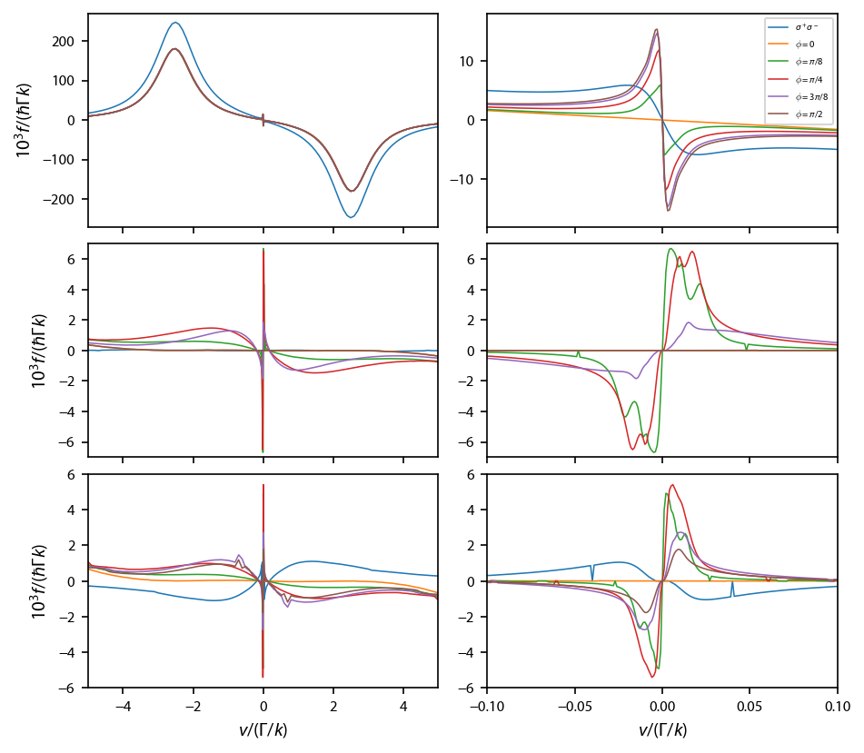
The results agree very well with Devlin, et. al., with the exception of a few glitches in the type-II molasses where the convergence criterion for the equilibrium force clearly failed.